Introduction
Dear Software Engineering Students,
Welcome to the CSF101 Class Notes Repository!
This repository serves as a comprehensive collection of all the class notes, exercises, and instructions for the CSF101 course. Whether you're a student looking to review previous lessons you'll find everything you need right here.
All the class notes are organized by topic, making it easy for you to navigate through the material. The course is divided into several units, each covering a different aspect of computer science and programming.
You will be tasked to complete all of the exercises provided in the class notes to reinforce your understanding of the concepts covered in the course and push to your github repo
- These exercises are designed to help you practice and apply what you've learned in a hands-on manner.
Feel free to explore the various folders and files within this repository to access the class notes for each topic covered in the course. Each set of notes is accompanied by exercises and clear instructions to help you reinforce your understanding of the material.
We hope that this repository will serve as a valuable resource throughout your CSF101 journey.
Happy learning!
CSF101 - Programming Methodology (Module Descriptor)
Programme: BE in Software Engineering
Credit: 12
Module Tutor: Sonam Yangchen
Module Coordinator: Douglas Sim
General Objective
This module introduces students to the fundamental concepts of programming and computational thinking. Starting with the foundations of computing and digital logic, the module progresses through programming fundamentals, data structures, and algorithms. Students will gain a comprehensive understanding of how computers process information, how to implement simple algorithms, and the process of formulating solutions using pseudocode and flowcharts.
Learning outcomes
On completion of this module, the students will be able to:
- Explain fundamental concepts in computing, including binary number systems, boolean logic, and basic computer architecture components.
- Convert between decimal and binary number systems, and perform basic binary operations.
- Analyze and design algorithms using pseudocode and flowcharts to solve computational problems.
- Implement basic programming constructs such as variables, operators, conditional statements, loops, and functions.
- Apply file operation methods to read from and write to files.
- Implement abstract data structures such as trees, graphs, stacks, queues, and linked lists using arrays.
- Implement and compare the efficiency of different searching and sorting algorithms on abstract data structures.
- Analyze the time and space complexity of algorithms using Big O notation.
- Apply graph traversal algorithms to solve pathfinding problems.
- Implement dynamic programming solutions for optimization problems.
Learning and teaching approach
| Type | Approach | Hours/week | Credit hours |
|---|---|---|---|
| Contact | Lecture | 2 | 30 |
| Practical | 2 | 30 | |
| Independent Study | Assignment | 2 | 30 |
| Self-study | 2 | 30 | |
| Total | 8 | 120 |
Assessment Approach
Assessment components consist of Continuous Assessment (CA) Theory - 60% and Continuous Assessment (CA) Practical - 40%. The CA Theory will consist of a Mid-Term test (15%), Assignment (30%), Quiz (15%), and CA Practical consists of Whiteboarding.
A. Mid-term Test: (15%)
Students will take a closed book written exam of a 2-hour duration covering subject matter from Unit-I to Unit-III. The exam will be marked out of 15 marks.
B. Programming Assignment: (30%)
The students will be given two programming assignments during the 7th and 12th week. Each assignment will be for 15 marks.
Programming Assignment I
Solve a programming problem using programming constructs, simple data structures, and algorithms. The assignment will be evaluated according to the following criteria:
- 2 Handling of input file
- 5 Time & Space Complexity Analysis
- 3 Code quality and readability
- 5 Implementation of appropriate data structures and algorithms
Programming Assignment II
Solve a programming problem using the concepts of dynamic programming:
- 2 Handling of input file
- 5 Time & Space Complexity Analysis
- 3 Code quality and readability
- 5 Implementation of appropriate data structures and algorithms
C. Quiz: (10%)
The students will be required to attempt two closed-book quizzes. Quiz one will test the student's understanding of the subject matter from Unit III and Quiz two will test the student's understanding of the subject matter from Unit IV. Each quiz will be conducted out of 10 marks each for one hour.
D. Practical Work & Report: (10%)
On completion of each weekly practical, a student is required to submit a weekly lab report with an executable file of the practical before the start of the subsequent practical class on a GitHub repository. The report will be written in markdown and submitted along with the executable file for which the format and instructions will be provided by the module tutor. Each report will be evaluated as per the following criteria:
- 3 Executability of the submission file without errors
- 2 Compliance with the instruction document
- 2 Solution approach
- 2 Use of adequate data structure and algorithm
- 1 Timely submission
E. Whiteboarding: (35%)
Students will participate in a whiteboarding assessment that consists of two parts: a Written Test and a Viva Voce. This examination will assess the student's ability to solve programming problems, explain their thought process, and optimize their solutions. The examination will be conducted in the 15th Week.
A. Written Test: (10%)
Each student will take a closed-book practical test for 1 hour where the students solve a specific programming problem. The test will be assessed based on the following criteria:
- 5 Pseudocode
- 5 Flowchart
B. Viva Voce: (25%)
Following the Practical Test, students will participate in a whiteboarding exercise where they will explain their solution approach for the question they solved in the practical test. They will also be asked to justify their solution methods and discuss potential optimizations. The assessment criteria for the Viva Voce are as follows:
- 3 Problem Comprehension
- 8 Technical Implementation
- 6 Solution Approach
- 4 Space/Time Analysis
- 4 Optimizations
Overview of the assessment approaches and weighting
| Areas of Assessment | Quantity | Weighting (%) |
|---|---|---|
| A. Mid-term Test | 1 | 15 |
| B. Programming Assignment | 2 | 30 |
| C. Quiz | 2 | 10 |
| D. Practical Work & Report | 9 | 10 |
| E. Whiteboarding | 1 | 35 |
| Total | 15 | 100 |
Pre-requisites
None
Subject matter
Unit I: Foundations of computing and digital logic
1.1 Introduction to computing
1.2 Information representation
   1.2.1 Bits and binary numbers
   1.2.2 Binary, octal, and hexadecimal number systems
   1.2.3 Two's complement representation
   1.2.4 Binary operations (addition and subtraction)
   1.2.5 Half adders and full adders
   1.2.6 Multi-bit addition
1.3 Character encoding
   1.3.1 ASCII standard
   1.3.2 Unicode and UTF-8
1.4 Boolean logic and logic gates
   1.4.1 Basic logic gates: AND, OR, NOT
   1.4.2 Composite logic gates: NAND, XOR
1.5 Introduction to Computer Architecture
   1.5.1 Von Neumann Architecture
   1.5.2 Harvard Architecture
Unit II: Programming Fundamentals
2.1 Evolution of programming languages
   2.1.1 Machine language, assembly language, and high-level languages
   2.1.2 Paradigms: imperative, declarative and functional
2.2 Compilers and interpreters
2.3 Computational problem solving
   2.3.1 Pseudocode
   2.3.2 Flowcharts
   2.3.3 Stepwise refinement and top-down design
2.4 Variables and Data Types
   2.4.1 Primitive data types
   2.4.2 Composite/Compound data types
   2.4.3 Type conversion and type casting
2.5 Operators
   2.5.1 Arithmetic operators
   2.5.2 Unary operators
   2.5.3 Assignment operators
   2.5.4 Comparative operators
   2.5.5 Logical operators
   2.5.6 Bitwise operators
   2.5.7 Conditional operators
2.6 Control structures
   2.6.1 Conditional statements (if-else, switch-case)
   2.6.2 Loops (for, while)
   2.6.3 Break and continue statements
2.7 Functions and Scope
   2.7.1 Function definition and invocation
   2.7.2 Parameters and return values
   2.7.3 Local and global scope
   2.7.4 Function Call Stack & Recursion
2.8 Memory Addresses & Pointers
2.9 File operations
   2.9.1 File input/output
   2.9.2 Text and binary file handling
Unit III: Data Structures
3.1 Introduction to storing data
   3.1.1 Static vs dynamic data structures
3.2 Elementary data structures
   3.2.1 Array and its properties
   3.2.2 Array operations and methods
   3.2.3 Multi-dimensional arrays
3.3 Linear Data Types
   3.3.1 List Abstract Data Structure (ADT)
   3.3.2 Stack, Queue, and Deque ADTs in their Linked List Implementations
   3.3.3 Stack and Queue in their (resize-able/circular) Array implementations
3.4 Linked structures
   3.4.1 Singly linked lists
   3.4.2 Doubly linked lists
   3.4.3 Circular linked lists
3.5 Tree data structures
   3.5.1 Binary trees and their properties
   3.5.2 Binary search trees (BST)
      3.5.2.1 BST properties and structure
      3.5.2.2 BST operations: insert, delete, search
      3.5.2.3 Tree traversals: in-order, pre-order, post-order
3.6 Graph data structures
   3.6.1 Graph representations: adjacency matrix and adjacency list
   3.6.2 Weighted and unweighted graphs
   3.6.3 Directed and undirected graphs
3.7 Table/Map ADT Concept
   3.7.1 Definition and Operations
   3.7.2 Unordered map characteristics
   3.7.3 Applications of unordered maps
3.8 Hash Table Implementation
   3.8.1 Hash function design
   3.8.2 Collision resolution: chaining
   3.8.3 Collision resolution: open addressing
   3.8.4 Dynamic resizing and rehashing
Unit IV: Searching & Sorting Algorithms
4.1 Linear Search
   4.1.1 Linear Search algorithm and implementation
   4.1.2 Time and space complexity
4.2 Binary Search
4.3 Depth-First Search (DFS)
   4.3.1 DFS algorithm and implementation
   4.3.2 DFS tree and edge classification
   4.3.3 Time and space complexity
   4.3.4 Applications: cycle detection, topological sorting
4.4 Breadth-First Search (BFS)
   4.4.1 BFS algorithm and implementation
   4.4.2 BFS tree and level order traversal
   4.4.3 Time and space complexity
4.5 Insertion Sort
4.6 Quick Sort
4.7 Bubble Sort
Unit V: Introduction to Computational Problems & Strategies
5.1 Space & Time Complexity, Asymptotic Notation
   5.1.1 Understanding space complexity
   5.1.2 Understanding time complexity
   5.1.3 Big O notation
   5.1.4 Omega and Theta notations
   5.1.5 Analyzing algorithm efficiency
   5.1.6 Comparing algorithm efficiencies
5.2 Arrays & Hashing
   5.2.1 Contains Duplicate problem
   5.2.2 Valid Anagram problem
   5.2.3 Two Sums problem
   5.2.4 Hash table implementations
   5.2.5 Collision resolution techniques
5.3 Two Pointers
   5.3.1 Valid Palindrome problem
   5.3.2 Three Sums problem
   5.3.3 Two pointers technique for array manipulation
   5.3.4 Applications in string problems
5.4 Sliding Window
   5.4.1 Best Time to Buy And Sell Stock problem
   5.4.2 Longest Substring Without Repeating Characters problem
   5.4.3 Fixed-size sliding window technique
   5.4.4 Variable-size sliding window technique
5.5 Stacks & Queues
   5.5.1 Valid Parentheses problem
   5.5.2 Implement Stack using Queue(s) problem
   5.5.3 Stack implementations and applications
   5.5.4 Queue implementations and applications
5.6 Linked List
   5.6.1 Reverse Linked List problem
   5.6.2 Merge Two Sorted Lists problem
   5.6.3 Remove Nth Node From End of List problem
   5.6.4 Singly and doubly linked list operations
5.7 Recursions
   5.7.1 Climbing Stairs problem
   5.7.2 Tower of Hanoi problem
   5.7.3 Understanding recursive algorithms
   5.7.4 Tail recursion optimization
5.8 Bit Manipulation
   5.8.1 Number of 1 Bits problem
   5.8.2 Counting Bits problem
   5.8.3 Reverse Bits problem
   5.8.4 Missing Numbers problem
   5.8.5 Bitwise operations and their applications
List of Practical(s)
- Implement a decimal-to-binary converter and basic logic gate simulator
- Create a text file analyzer that calculates various statistics using control structures
- Implement recursive and iterative Fibonacci sequence generators
- Implement linear and binary search algorithms
- Implement stack and queue data structures and use them to solve practical problems
- Create a singly linked list with basic operations and list manipulation functions
- Implement a binary search tree with insertion, deletion, search, and traversal operations
- Implement bubble, merge, and quick sort algorithms
- Create a graph data structure and implement basic graph traversal algorithms
Reading list
Essential Reading
- Cormen, T. H., Leiserson, C. E., Rivest, R. L., & Stein, C. (2022). Introduction to Algorithms, fourth edition. MIT Press.
- Abelson, H. (1996). Structure and interpretation of computer programs. Mit Press.
- Bryant, R. E., & O'Hallaron, D. R. (2015). Computer systems: A Programmer's Perspective, Global Edition.
Additional Reading
- Simpson, K. (2020). You don't know JS yet: Get Started.
- Haverbeke, M. (2018). Eloquent JavaScript, 3rd Edition: A Modern Introduction to Programming. No Starch Press.
Date: August 2024
Git & GitHub for Beginners
Introduction to Git
Git is a distributed version control system that helps developers track changes in their code, collaborate with others, and manage different versions of their projects. It's an essential tool for modern software development, especially when working in teams or on open-source projects.
Setting Up Git
Before you start using Git, you need to install it and configure your identity:
- Linux users can install Git using their package manager (e.g.,
sudo apt install git) - Windows users can download git using
choco install git. - Mac users can install Git using
brew install git - Open a terminal or command prompt
- Set your name and email (used for commit messages):
git config --global user.name "Your Name"
git config --global user.email "your.email@example.com"
Creating a repository in GitHub

Basic Git Commands
Initializing a Repository
To start tracking a project with Git, navigate to your project directory and run:
git init
This creates a new Git repository in your current directory.
Checking Repository Status
To see the current state of your repository:
git status
This command shows which files have been modified, staged, or are untracked.
Adding Files to the Staging Area
To prepare files for commit, you need to add them to the staging area:
# Add a specific file
git add filename.txt

# Add all files in the current directory
git add .

# Add all files with a specific extension
git add *.js
Committing Changes
To save your staged changes to the repository:
git commit -m "Your commit message here"
For a more detailed commit message, omit the -m flag:
git commit
This will open your default text editor where you can write a multi-line commit message.
Viewing Commit History
To see the history of commits:
# View all commits
git log

# View a condensed version of the log
git log --oneline

# View the last 5 commits
git log -n 5
Working with Remote Repositories (GitHub)
Cloning a Repository
To create a local copy of a remote repository:
git clone https://github.com/username/repository.git
Adding a Remote Repository
If you've created a local repository and want to link it to a GitHub repository:
git remote add origin https://github.com/username/repository.git
Pushing Changes to GitHub
To send your local commits to the remote repository:
# First time push (sets up tracking)
git push -u origin main

# Subsequent pushes
git push
Pulling Changes from GitHub
To fetch and merge changes from the remote repository:
git pull
This is equivalent to running git fetch followed by git merge.
Branching
Branches allow you to work on different features or versions of your project simultaneously.
Creating a New Branch
git branch new-feature
Switching to a Branch
git checkout new-feature
Or, create and switch to a new branch in one command:
git checkout -b another-feature
Merging Branches
To merge changes from one branch into another:
# First, switch to the branch you want to merge into
git checkout main

# Then merge the feature branch
git merge new-feature
Handling Merge Conflicts
Sometimes Git can't automatically merge changes, and you'll need to resolve conflicts manually:
- Open the conflicting file(s) in your text editor
- Look for the conflict markers (
<<<<<<<,=======,>>>>>>>) - Edit the file to resolve the conflict
- Save the file
- Stage the resolved file:
git add filename.txt - Complete the merge by committing:
git commit -m "Resolved merge conflict"
Undoing Changes
Discard Changes in Working Directory
git checkout -- filename.txt
Unstage a File
git reset HEAD filename.txt
Amend the Last Commit
git commit --amend
This opens your editor to modify the commit message. If you've staged changes, they'll be added to the amended commit.
Best Practices
- Commit often: Make small, focused commits that are easy to understand and review.
- Write clear commit messages: Briefly describe what changes were made and why.
- Use branches for new features or experiments.
- Pull changes from the remote repository before starting new work to avoid conflicts.
- Review your changes before committing: Use
git diffto see what you've modified.
Online Resources for Further Exploration:
- Learn Git Branching - Online Visual Game
- Git Tutorial - Git Docs
- Concepts of all the git commands - Git Kraken
Introduction To Computing
The word computer derives from the word compute which means to calculate. The history of computers which are devices used to calculate and do simple arithmetic operation dates all the way back to ancient China where abacus was used to perform basic mathematical operations fast and efficicently. They were also often used to store the results of such operations.

A model of one of the world's first computers (the Difference Engine invented by Charles Babbage) at the Computer History Museum in Mountain View, California, USA
History
While the evolutionary journey of computing is fascinating, its concerns lie beyond the scope of the syllabus, but feel free to read more about it here. What cocnerns us most now is the invention of Mark I in 1944 by Dr. Howard Aiken and Grace Hopper. This is said to be a crucial landmark for the world of computing as Mark I was considered to be worlds first electormechanical computer capable of making logical decisions.
Today
Our second point of concern is invention of transistors in 1948 at Bell Labs which forever changed the course of computers and modern day electronics. Ever since these signifcant milestones, computers have become smaller and faster as described by the Moores Law.Today, we use hand held devices with the computing power which is atleast 100,000 times more than what was used to send the Apollo 11 mission to the moon.
Tomorrow
But what is in store for us tomorrow? With the growth of AI industry and improvements in GPU compute, we are pushing the limits of computing as well as data to an unimaginable scale. With the potential of quantum computers still in the horizon the future of computers sure is promising. I hope that throughout the course of this module, we are able to give you a good feel of what computers are, what they are capable of and how you can use them to your advantage for years to come.
Note: Dont be concerned if the terms and concepts discussed in these articles seem concerning, we will discuss the key concepts in class.
Information Representation
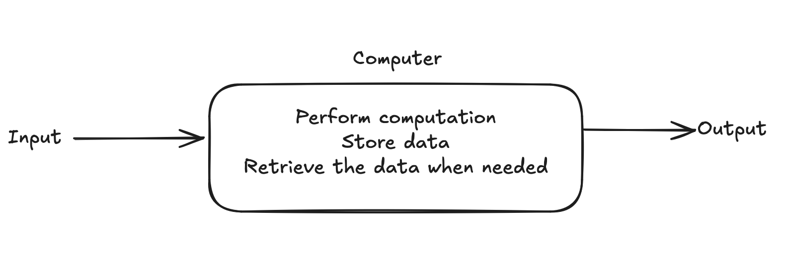
An over simplified definition of a computer would be a device that can recieve input, process this input to do some computation, store necesarry data, and retrieve this data to present an output when needed. We will discuss more about various parts of a computer and their unqiue functions in the later part of the chapter, but for now we, will take a bottom-up approach of learning the fundamental components that makes up a computer.
For this topic, we are to understand the following key concepts:
- How does a computer store data?
- Where does a computer store data?
- What format does a computer store data in?
- How does a computer perform basic airthmetic operations with this stored information?
1.2.1 Bits and Binary numbers.
Computers are made up of millions of small electronic devices. These devices are responsible for representing information, performing calculations and storing information and while these functions seem distinctly different from each other, the parts that perform these functions are all made up of the same fundamental electronic components in different configurations.
Bits
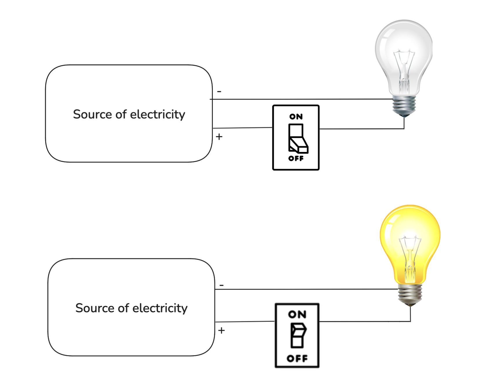
Imagine a light bulb that is connected to a single switch. When the switch is turned on the bulb lights up and when it is turned off the bulb turns off. A lightbulb in this case can represent two states of either being on or off. We can then go ahead and label the off state of a light bulb to be 0 and the on state to be 1. A bulb can only have two possible states in this analogy and we can proceed to describe the nature of states of a light bulb to be binary.
Similar to this imaginary light bulb, computer are made up of millions of parts that function similar to the aforementioned switches, where a bit may represent 0 or 1. Note that one bit can represent only two states, however if two bits are placed side by the side, they can represent 4 states in combination as shown in the graphic below.
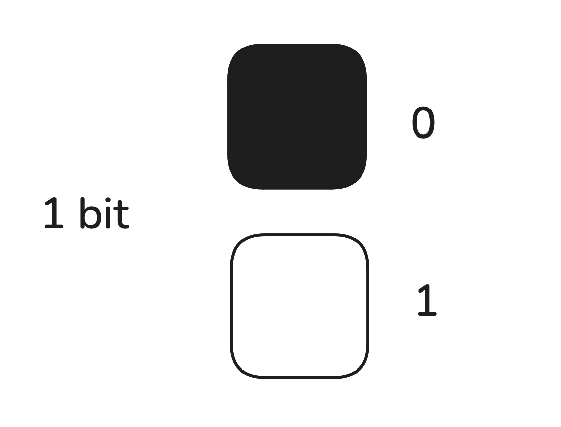
Fig: one bit represents two states
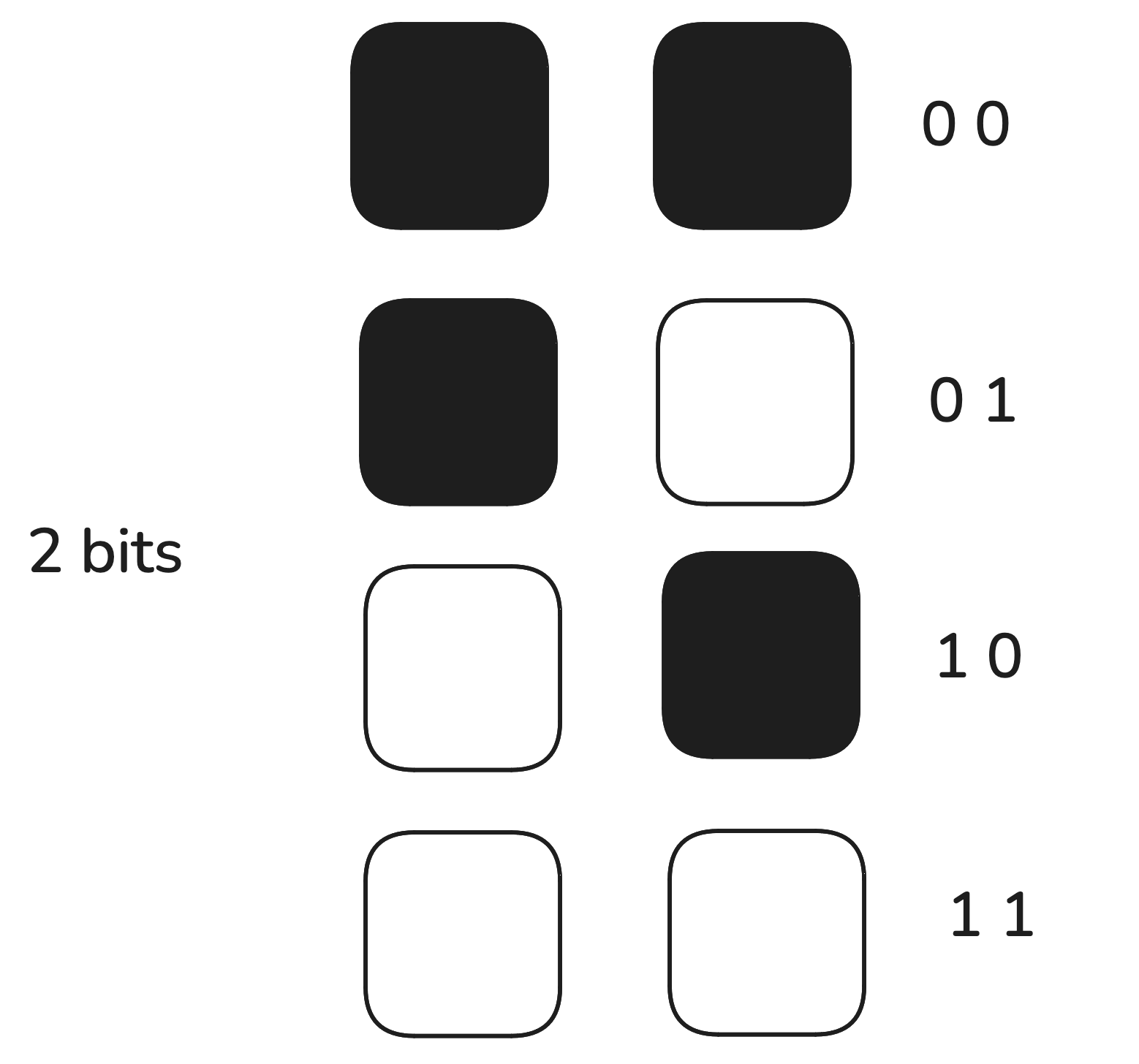
Fig: two bits represents four states
Similarly many bits can be used to represent many states, note that if the number of bits used is equal to n, the total number of states a combination of n bits can represent can be calculcated as 2n(where n>=1 and cannot be 0, negative or a fraction).
Binary Number System
This positional number system which represents numbers using 0's and 1's is known as the binary number system.The following table highlights number of bits and its relation to number of states the bits can represent:
| No of bits | No of States |
|---|---|
| 1 | 2 |
| 2 | 4 |
| 3 | 8 |
| 4 | 16 |
| 5 | 32 |
| 6 | 64 |
| 7 | 128 |
| 8 | 256 |
Storage
In practise, when storing information the term byte is often used which represents a total of 256 states (23) which can be represented by a combination of 8 bits. Meaning 1 byte consists of 256 possible states and one byte of information represets one such state, Similarly other units of measurements are as stated in the table below:
| Units of measurement | Experession in powers of 2 |
|---|---|
| Byte | 23 |
| Kibibyte(KiB) | 210 |
| Mebibyte(MiB) | 220 |
| Gigibyte(GiB) | 230 |
| Tebibyte(TiB) | 240 |
| Pebibyte(PiB) | 250 |
There is a variation in how size of data is representation in terms of binary and decimal number systems. For marketing and generic purposes, the terms such as Kilobytes, Megabytes and Gigabytes are used more often. You can read more about his in the official IBM article here.
1.2.2 Binary, Octal, and Hexadecimal, Number systems
A number can be represented with different base values. We are familiar with the numbers in the base 10 (known as decimal numbers), with digits taking values 0,1,2,…,8,9
A computer uses a Binary number system which has a base 2 and digits can have only TWO values: 0 and 1.
A decimal number with a few digits can be expressed in binary form using a large number of digits. Thus the number 65 can be expressed in binary form as 1000001.
The binary form can be expressed more compactly by grouping 3 binary digits together to form an octal number. An octal number with base 8 makes use of the EIGHT digits 0,1,2,3,4,5,6 and 7
A more compact representation is used by Hexadecimal representation which groups 4 binary digits together. It can make use of 16 digits, but since we have only 10 digits, the remaining 6 digits are made up of first 6 letters of the alphabet. Thus the hexadecimal base uses 0,1,2,….8,9,A,B,C,D,E,F as digits.
The table below shows how different number represents different number:
| Decimal | Binary | Octal | Hexadecimal |
|---|---|---|---|
| 0 | 0000 | 0 | 0 |
| 1 | 0001 | 1 | 1 |
| 2 | 0010 | 2 | 2 |
| 3 | 0011 | 3 | 3 |
| 4 | 0100 | 4 | 4 |
| 5 | 0101 | 5 | 5 |
| 6 | 0110 | 6 | 6 |
| 7 | 0111 | 7 | 7 |
| 8 | 1000 | 10 | 8 |
| 9 | 1001 | 11 | 9 |
| 10 | 1010 | 12 | A |
| 11 | 1011 | 13 | B |
| 12 | 1100 | 14 | C |
| 13 | 1101 | 15 | D |
| 14 | 1110 | 16 | E |
| 15 | 1111 | 17 | F |
1.2.2 Twos complement representation
The twos complement method is a common way to represent signed integers in computers. It is also often used to simplify binary operations as its used to represent negative numbers in binary. The steps for twos complement method are as follows:
- Step 1: Start with the absolute binary representation of a number
- Step 2: Ivert all bits (change 0's to 1s and vice vaersa)
- Step 3: Add 1 to this representation
The way twos complement method can be used to represent negative integers as explained in this handout.
1.2.3 Binary operations
Similar to how we perform arithmetic operations such as addition and subtraction in decimal number system, we can do the same for binary numbers. For binary addition, the binary representation of both the numbers are to be placed in a cascade such that both binary representations have equal number of digits. Once this is done the digits can be compared from the position of least significant bit(right most) with the following rules:
- Rule 1: 0 + 0 = 0
- Rule 2: 0 + 0 = 1
- Rule 3: 1 + 0 = 1
- Rule 4: 1 + 1 = 0 (carry)
Similarly for binary subtraction:
- Rule 1: 0 - 0 = 0
- Rule 2: 1 - 0 = 1
- Rule 3: 0 - 1 = 1 (borrow)
- Rule 4: 1 - 1 = 0
Note that multiplication and division are just repeated addition and subtraction respectively. Examples of binary addition and subtraction operations are available in the following video.
While the above mentioned rules for binary subtraction is applicable, computers compute differences using the two's complements method. Therefore for binary subtraction using the two's complement method:
- Step 1: take the binary representation of two numbers to be subtracted.
- Step 2: identify the two's complement representation of the subtrahend
- Step 3: add the binary representation of the initial number to the two's complement representation of the subtrahend.
- Step 4: discard the most signifcant bit of the solution
Essential resources:
- Half adders and full adder : LINK
- Binary adder implementation using full adders : LINK
- Binary subtractor implementation using full adders : LINK
Additional Resources
Character Encoding
1.3.1 The ASCII standard
With the understanding of binary and how it can be used to represent many states in combination, it is now important to understand how binary represents different characters in a computer. We can group characters into three main groups i.e. alphabetic characters (a z and A to Z), numeric characters (0-9) and special characters ($,%,#,@ etc).
ASCII is an international standard which stands for American Standard Code for Information Interchange, which is a character encoding standard for almost all electronic communication. The chart below provides a visualization of how these characters are represented in binary and what is the equivalent decimal representation for each unique character.
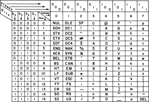
ASCII chart (1972)
The standard ASCII characters which adds up to 126 unique characters can be represented using 7 bits. However an extended version of the ASCII table called the extended ASCII can represent up to 256 characters using 8 bits.
Excercise: Use the standard ASCII table to write your full name.
1.3.2 Unicode and UTF8 encoding
While the ASCII table was enough to represent basic alphanumeric characters and few special characters, the computers today have to store other characters such as emojis and characters from different languages. This is not simple as there are many languages with different structures, some languages use alphabets, vowels, and consonants while some langauges use strokes and other form of expression to represent different characters.
Unicode is one such standard that tries to solve the problem of storing and representing different characters in a computer. While each character is mapped to a bit representation, unicode uses codepoints where different characters are mapped to uniique hexadecimal digita. This representation is made as U+XXXX where U+ means unicode and the XXXX represents hexadecimal numbers.
The UTF-8 encoding scheme was later developed to ensure that no extra bit space is consumed while representing characters. UTF-8 representation of characters for english is very similar to that of the ASCII table where it only uses one byte(8 bits) or two hexadecimals to represent characters. However, however for more than 127 characters, several bytes are used to represent the characters. You can read more about this in the following articles and official documentation:
1.4 Boolean logic and Logic gates
1.4.1 Basic logic gates
The expression of values in binary which uses 0's and 1's can also be used to experess simple logic such as true or false. Computers first used the binary number system as there was an entire branch of mathematics that dealt with representaition and manipulation of true and falase values known as the boolean algebra. The mathematical analysis of logic book written by George Boole in 1847 states that boolean algebra allows for truth to be systematically and formallly proven through logic equations.
There are three fundamental operations used in boolean algebra known as the AND, OR and the NOT operation. Note that these operations were later simulated into electrical components using transistors and are called logic gates which follow their respective properties as expressed in boolean algebra. A detailed video on this concept can be found here.
Transistors are electrically controlled switches whereby, when an adequate amount of electricity flows through one of the input electrode(base), the transistors allows electricity to flow through the other two electrodes(collector to emitter) as shown in the graphic below.
A simple transistor
We can represent various logic gates using truth tables. The AND and OR gates can be represented as shown below:
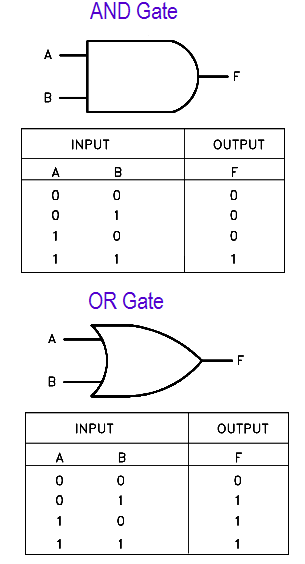
Truth tables for AND and OR gates
A NOT gate takes in one input and flips it to its reverse state therefore its truth table is as shown below:
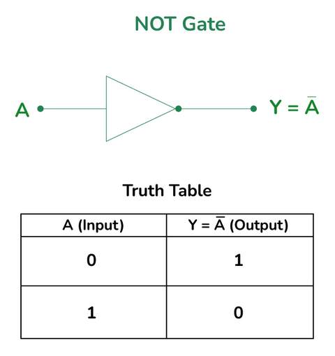
NOT gate
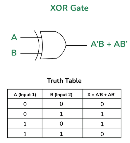
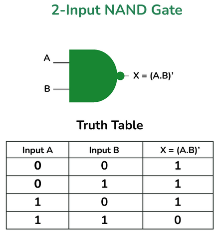
1.2.2 Composite logic gate
There are other logic gates that prove to be very useful in computers when applying more complex computations. One such example is use of logic gates to perform binary addition and subtraction. The NAND gate in particular is very important as it is also often termed as the universal gate as it can be used to constructure AND, OR and NOT gates when placed in a certain configuration.
Similarly the XOR gate is important as it is used for arithmetic computation. This can be observed in the networking module where XOR logic is used to do error checking and binary addition. There truth tables and symbols are as follows:
1.5 Introduction to computer architecutre
Over the course of many generations in advancement of computers and technology, there has been various improvements with regard to different parts of a computer. A brief history of these generation can be found in this article.
The modern day computers have very distinct parts with specialized functions. At a high level, a computer can be escribed using the following diagram:

Block diagram of a computer
Different parts of a computer and its functions
- Central Processing Unit (CPU)
- Executes instructions and performs calculations
- Key components:
- Control Unit: Manages and coordinates CPU operations
- Arithmetic Logic Unit (ALU): Performs arithmetic and logical operations
- Registers: Small, fast storage locations within the CPU
- Memory
- A physical device that stores information temporarily or permanently.
- Provides quick access to data and instructions for the CPU, act as a speed buffer, serve as an active workspace, and hold temporary data
- The two main types include:
- Random Access Memory (RAM):
- Volatile memory used for temporary data storage
- Faster access times compared to storage devices
- Read-Only Memory (ROM):
- Non-volatile memory containing essential instructions (e.g., BIOS)
- Random Access Memory (RAM):
- Storage devices
- These devices stores data into devices such as drives or disks.
- Solid state drives (SSD) and Hard disk drives(HDD) are most commonly used.
- Input/Output devices (I/O)
- Input: Keyboard, mouse, microphone, camera
- Output: Monitor, speakers, printer
- Bus systems
- Provides connection and enables communication between different parts of a computer
- Data Bus: Transfers data between components
- Address Bus: Carries memory addresses
- Control Bus: Carries control signal
The Fetch-Decode-Execute Cycle
The fetch-decode-execute cycle (also known as the instruction cycle) is the basic operational process of a computer. It's the sequence of steps that the CPU follows to process each instruction in a program.
- Fetch
- The CPU retrieves (fetches) an instruction from memory.
- This instruction is stored in a special register called the Instruction Register (IR).
- The Program Counter (PC) keeps track of which instruction to fetch next.
- Decode
- The CPU interprets (decodes) the instruction.
- It figures out what operation needs to be performed.
- For example, it might be an addition, a memory access, or a jump to another part of the program.
- Execute
- The CPU carries out (executes) the instruction.
- This might involve:
- Performing a calculation
- Moving data
- Changing the sequence of instructions (in case of a jump)
1.5.1 Von Neumann Architecture
Both Harvard and von Neumann architectures are fundamental designs for computer systems, each with its own approach to handling program instructions and data. Understanding these architectures helps in grasping how different computer systems implement the fetch-decode-execute cycle.
Key Characteristics:
- Single memory space for both data and instructions
- Uses a single bus for both data and instruction transfer
Fetch-Decode-Execute in von Neumann:
- Fetch: Instructions and data are fetched from the same memory.
- Decode: The CPU decodes the instruction.
- Execute: The CPU executes the instruction, potentially accessing the same memory for data.
Advantages:
- Simpler design
- Flexible use of memory (can allocate more space to either instructions or data as needed)
Disadvantages:
- Potential bottleneck due to single bus (known as the von Neumann bottleneck)
- Instructions and data compete for memory access
1.5.2 Harvard Architecture
Key Characteristics:
- Separate memory spaces for instructions and data
- Uses separate buses for instruction and data transfer
Fetch-Decode-Execute in Harvard:
- Fetch: Instructions are fetched from instruction memory.
- Decode: The CPU decodes the instruction.
- Execute: The CPU executes the instruction, accessing data memory if needed.
Advantages:
- Can fetch next instruction and access data simultaneously
- Potentially faster execution due to parallel access
- Better security (can make instruction memory read-only)
Disadvantages:
- More complex design
- Fixed allocation of memory between instructions and data
Comparison in Context
-
Memory Access:
- von Neumann: One memory access per cycle (either instruction or data)
- Harvard: Can perform instruction fetch and data access in the same cycle
-
Parallelism:
- von Neumann: Limited by single bus
- Harvard: Allows for more parallelism in instruction processing
-
Impact on Fetch-Decode-Execute Cycle
- von Neumann: The cycle may be slowed down when instruction fetch and data access compete for the same memory bus.
- Harvard: The cycle can potentially be faster as instruction fetch doesn't compete with data access.
Modern Implementations:
Many modern CPUs use a modified Harvard architecture, with separate caches for instructions and data, but a unified main memory (like von Neumann)
Psuedocode
1. Introduction to Pseudocode
Pseudocode is a method of describing algorithms in a structured, readable format that is close to a programming language but is not tied to any specific language syntax.
It allows algorithm designers to express ideas clearly without getting bogged down in language-specific details.
2. Key Principles of Pseudocode
2.1 Clarity and Readability
Pseudocode should be easy to read and understand, even for those not familiar with specific programming languages.
2.2 Precision
While not as strict as actual code, pseudocode should be precise enough to be translated into a programming language without ambiguity.
2.3 Abstraction
Pseudocode allows for a higher level of abstraction than actual code, focusing on the logic rather than implementation details.
3. Common Pseudocode Conventions
3.1 Indentation
Use indentation to show the structure and nesting of control structures.
3.2 Keywords
Use keywords like IF, ELSE, WHILE, FOR, RETURN in uppercase for clarity.
3.3 Comments
Use // for single-line comments and /* */ for multi-line comments.
4. Basic Structures in Pseudocode
4.1 Assignment
x = 5
4.2 Input/Output
READ x
PRINT "The value is:", x
4.3 Conditional Statements
IF condition THEN
    statement1
    statement2
ELSE
    statement3
ENDIF
4.4 Loops
// While Loops
WHILE condition DO
    statement1
    statement2
ENDWHILE

// For Loops
FOR i = 1 TO n
    // statements
ENDFOR
4.5 Functions
FUNCTION FunctionName(parameter1, parameter2)
    // statements
    RETURN value
ENDFUNCTION
5. Example Pseudocode Algorithms
5.1 Linear Search
ALGORITHM LinearSearch(A, n, x)
    INPUT: An array A of n elements and a value x
    OUTPUT: Index of x in A or -1 if not found

    FOR i = 0 TO n - 1
        IF A[i] = x THEN
            RETURN i
        ENDIF
    ENDFOR
    RETURN -1
5.2 Binary Search
ALGORITHM BinarySearch(A, n, x)
    INPUT: A sorted array A of n elements and a value x
    OUTPUT: Index of x in A or -1 if not found

    left = 0
    right = n - 1
    WHILE left ≤ right DO
        mid - ⌊(left + right) / 2⌋
        IF A[mid] = x THEN
            RETURN mid
        ELSE IF A[mid] < x THEN
            left = mid + 1
        ELSE
            right = mid - 1
        ENDIF
    ENDWHILE
    RETURN -1
5.3 Insertion Sort
ALGORITHM InsertionSort(A, n)
    INPUT: An array A of n elements
    OUTPUT: A sorted in ascending order

    FOR i = 1 TO n - 1
        key = A[i]
        j = i - 1
        WHILE j ≥ 0 AND A[j] > key
            A[j + 1] = A[j]
            j = j - 1
        ENDWHILE
        A[j + 1] = key
    ENDFOR
6. Advanced Pseudocode Techniques
6.1 Recursive Algorithms
Example: Factorial calculation
FUNCTION Factorial(n)
    IF n = 0 THEN
        RETURN 1
    ELSE
        RETURN n * Factorial(n - 1)
    ENDIF
7. Best Practices for Writing Pseudocode
- Be consistent in your style and notation.
- Use meaningful variable and function names.
- Include comments to explain complex logic.
- Use appropriate levels of abstraction.
- Revise and refine your pseudocode as you develop your algorithm.
Remember, the goal of pseudocode is to communicate algorithmic ideas clearly and effectively.
Flowcharts
1. Introduction to Flowcharts
Flowcharts are graphical representations of algorithms, workflows, or processes.
They use standardized symbols to illustrate the steps and decision points in a process, making it easier to visualize and understand complex procedures.
2. Key Principles of Flowcharts
2.1 Clarity and Readability
Flowcharts should be easy to follow and understand, even for those not familiar with the specific process being described.
2.2 Consistency
Use standardized symbols and follow consistent conventions throughout the flowchart.
2.3 Simplicity
Break down complex processes into simpler steps, using sub-processes where necessary to maintain clarity.
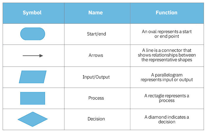
3. Standard Flowchart Symbols and Their Meanings
3.1 Oval (Terminal)
- Represents the start or end of a program or process.
- Typically contains "Start" or "End" text.
- Indicates the entry and exit points of a flowchart.
3.2 Arrow (Flow Line)
- Shows the direction of process flow.
- Connects different elements of the flowchart.
- Indicates the sequence of operations.
3.3 Parallelogram (Input/Output)
- Represents input or output operations.
- Used for displaying data entry or results.
- Can indicate manual input, printed output, or displayed information.
3.4 Rectangle (Process)
- Represents a processing step or action.
- Indicates any operation where data is manipulated or changed.
- Can represent calculations, data transformations, or function calls.
3.5 Diamond (Decision)
- Represents a decision point or branching in the process.
- Contains a question or condition that can be answered with "Yes" or "No" (True or False).
- Has two outgoing arrows, typically labeled with the possible outcomes.
4. Tools for Creating Flowcharts
Use any of the tools below to create flowcharts for your assignments:
- Exacalidraw
- FigJam
- Microsoft Visio
- Lucidchart
- Draw.io
- SmartDraw
- Creately
These tools provide templates and drag-and-drop interfaces for creating professional flowcharts.
Exercise
Create Flowcharts and Psuedocode for the following problems:
NOTE:
- For terms and topics you do not understand: Google to understand what they are.
- Most of the terms are important computing terms/problems
- You need to practise Googling
Level 1
- Calculate the area of a rectangle given its length and width.
- Determine if a number is even or odd.
- Find the largest of three given numbers.
- Convert temperature from Celsius to Fahrenheit.
- Calculate the sum of all numbers from 1 to n.
- Check if a given year is a leap year.
- Generate the first n terms of the Fibonacci sequence.
- Calculate the factorial of a given number.
- Determine if a given string is a palindrome.
- Find the average of n numbers.
- Convert a decimal number to binary.
- Check if a number is prime.
- Reverse a given string.
- Calculate the compound interest for a given principal, rate, and time.
- Find the GCD (Greatest Common Divisor) of two numbers.
- Convert a given number of days to years, weeks, and days.
- Generate a multiplication table for a given number.
- Calculate the power of a number (x^n).
- Find the smallest element in an array.
- Determine if a triangle is equilateral, isosceles, or scalene given its sides.
- Calculate the roots of a quadratic equation.
- Convert a given number of seconds to hours, minutes, and seconds.
- Find the number of vowels in a given string.
- Calculate the perimeter of a circle given its radius.
- Determine if a number is a perfect square.
- Generate all prime numbers up to n.
- Calculate the sum of digits of a given number.
- Find the LCM (Least Common Multiple) of two numbers.
- Check if a given number is a Armstrong number.
- Calculate the simple interest for a given principal, rate, and time.
Level 2
- Find the sum of all even numbers between 1 and n.
- Calculate the area of a triangle given its base and height.
- Determine if a number is positive, negative, or zero.
- Convert a binary number to decimal.
- Find the factors of a given number.
- Calculate the volume of a cube given its side length.
- Generate a sequence of n random numbers between 1 and 100.
- Find the maximum and minimum values in an array.
- Calculate the sum of squares of numbers from 1 to n.
- Determine if a given character is a vowel or consonant.
- Calculate the perimeter of a rectangle given its length and width.
- Find the number of occurrences of a specific digit in a given number.
- Generate a pattern of asterisks in the shape of a right-angled triangle.
- Calculate the average of numbers in an array, excluding the largest and smallest values.
- Determine if a given year is a century year.
- Find the sum of all odd numbers between two given numbers.
- Calculate the distance traveled given initial velocity, acceleration, and time.
- Generate the first n terms of an arithmetic sequence given the first term and common difference.
- Find the absolute difference between two numbers.
- Calculate the area of a circle given its diameter.
Level 3
- Implement a basic calculator that can handle multiple operations in one expression. (BEDMAS)
- Find the second largest and second smallest elements in an array.
- Check if a given password is strong based on criteria: length, inclusion of numbers, special characters.
- Calculate the Body Mass Index (BMI) and categorize it (underweight, normal, overweight, obese).
- Implement a basic Caesar cipher for encrypting and decrypting messages.
- Find the most frequent element in an array.
- Calculate the nth term of a geometric sequence.
- Implement a simple game of rock-paper-scissors against the computer.
- Convert a decimal number to its Roman numeral representation (up to 3999).
- Calculate the area of a regular polygon given the number of sides and side length.
Variables & Data Types
Variables and Data Types in Python
Variables are containers for storing data values. In Python, you don't need to declare variables before using them or declare their type.
Python automatically determines the variable's data type based on the value assigned to it.
1. Primitive Data Types
Python has several built-in primitive data types:
Integers (int)
Whole numbers, positive or negative, without decimals.
age = 25
temperature = -5
Floating-point numbers (float)
Numbers with decimal points or in exponential form.
pi = 3.14159
avogadro = 6.022e23  # Scientific notation
Strings (str)
Sequences of characters, enclosed in single or double quotes.
name = "Alice"
message = 'Hello, World!'
multiline = """This is a
multiline string."""
Booleans (bool)
Represents True or False values.
is_python_fun = True
is_raining = False
None
Represents the absence of a value or a null value.
result = None
2. Composite/Compound Data Types
Composite data types are collections of other data types:
Lists
Ordered, mutable sequences of elements.
fruits = ["apple", "banana", "cherry"]
mixed_list = [1, "two", 3.0, True]
Tuples
Ordered, immutable sequences of elements.
coordinates = (10, 20)
rgb = (255, 0, 128)
Dictionaries
Unordered collections of key-value pairs.
person = {
    "name": "Bob",
    "age": 30,
    "city": "New York"
}
Sets
Unordered collections of unique elements.
unique_numbers = {1, 2, 3, 4, 5}
vowels = set(['a', 'e', 'i', 'o', 'u'])
Type Conversion and Type Casting
Python allows you to convert between different data types:
Implicit Type Conversion
Python automatically converts one data type to another if needed.
x = 5
y = 2.0
result = x + y  # result will be a float (7.0)
Explicit Type Conversion (Type Casting)
You can manually convert between types using built-in functions.
# String to Integer
age_str = "25"
age_int = int(age_str)  # 25

# Integer to String
number = 42
number_str = str(number)  # "42"

# String to Float
price_str = "19.99"
price_float = float(price_str)  # 19.99

# Float to Integer (truncates decimal part)
height = 1.75
height_int = int(height)  # 1

# Integer to Float
count = 10
count_float = float(count)  # 10.0

# String to List
word = "Python"
char_list = list(word)  # ['P', 'y', 't', 'h', 'o', 'n']

# List to Set (removes duplicates)
numbers = [1, 2, 2, 3, 4, 4, 5]
unique_set = set(numbers)  # {1, 2, 3, 4, 5}
Remember that not all type conversions are possible, and some may result in loss of information or raise exceptions if the conversion is invalid.
Exercise
Exercises: Variables and Data Types
These exercises are designed to help you practice working with variables and different data types in Python. Follow each step carefully and try to predict the output before running the code.
File Organization
To keep your work organized, we'll use the following file structure:
csf101-python_exercises/
│
├── basics/
│   ├── numbers.py
│   ├── strings.py
│   └── booleans.py
│
└── data_structures/
    ├── lists.py
    └── dictionaries.py
Create a new directory called python_exercises and navigate into it. Then, create two subdirectories: basics and data_structures.
Exercise 1: Working with Integers and Floats
File: basics/numbers.py
Create a new file called numbers.py in the basics directory and complete the following exercises in this file.
-
Create a variable
ageand assign it your age as an integer.age = 25 # Replace with your actual age print(age)Expected output:
25 -
Create a variable
heightand assign it your height in meters as a float.height = 1.75 # Replace with your actual height print(height)Expected output:
1.75 -
Calculate your age in days (assume 365 days per year) and store it in a variable
age_in_days.age_in_days = age * 365 print(age_in_days)Expected output:
9125 -
Divide your
ageby 7 and print the result.result = age / 7 print(result)Expected output:
3.5714285714285716Note: The result is a float, even though we started with integers.
Exercise 2: Working with Strings
File: basics/strings.py
Create a new file called strings.py in the basics directory and complete the following exercises in this file.
-
Create a variable
nameand assign it your full name as a string.name = "John Doe" # Replace with your actual name print(name)Expected output:
John Doe -
Use string concatenation to create a greeting message.
greeting = "Hello, " + name + "!"
print(greeting)
Expected output:
Hello, John Doe! -
Use f-strings to create the same greeting message.
greeting_f = f"Hello, {name}!"
print(greeting_f)
Expected output:
Hello, John Doe! -
Print the length of your name.
name_length = len(name)
print(name_length)
Expected output:
8Warning: Remember that spaces count as characters too!
Exercise 3: Working with Booleans
File: basics/booleans.py
Create a new file called booleans.py in the basics directory and complete the following exercises in this file.
-
Create two boolean variables,
is_studentandis_employed, and assign them appropriate values.is_student = True is_employed = False print(is_student, is_employed)Expected output:
True False -
Use the
andoperator to check if you are both a student and employed.is_student_and_employed = is_student and is_employed print(is_student_and_employed)Expected output:
False -
Use the
oroperator to check if you are either a student or employed.is_student_or_employed = is_student or is_employed print(is_student_or_employed)Expected output:
True
Exercise 4: Type Conversion
File: basics/type_conversion.py
Create a new file called type_conversion.py in the basics directory and complete the following exercises in this file.
-
Convert your
ageto a string and concatenate it with a message.age = 25 # Use the same age as in numbers.py age_str = str(age) message = "I am " + age_str + " years old." print(message)Expected output:
I am 25 years old. -
Try to convert a string to an integer.
num_str = "42"
num_int = int(num_str)
print(num_int)
Expected output:
42 -
Now try to convert a non-numeric string to an integer.
non_num_str = "Hello"
try:
    non_num_int = int(non_num_str)
    print(non_num_int)
except ValueError as e:
    print(f"Error: {e}")
Expected output:
Error: invalid literal for int() with base 10: 'Hello'Note: This will raise a ValueError, which we catch and print.
Exercise 5: Working with Lists
File: data_structures/lists.py
Create a new file called lists.py in the data_structures directory and complete the following exercises in this file.
-
Create a list of your favorite fruits.
fruits = ["apple", "banana", "cherry"]
print(fruits)
Expected output:
['apple', 'banana', 'cherry'] -
Add a new fruit to your list using the
append()method.fruits.append("date") print(fruits)Expected output:
['apple', 'banana', 'cherry', 'date'] -
Access and print the second fruit in your list.
second_fruit = fruits[1]
print(second_fruit)
Expected output:
bananaWarning: Remember that list indices start at 0!
Exercise 6: Working with Dictionaries
File: data_structures/dictionaries.py
Create a new file called dictionaries.py in the data_structures directory and complete the following exercises in this file.
-
Create a dictionary with information about yourself.
name = "John Doe"  # Use the same name as in strings.py
age = 25  # Use the same age as in numbers.py
height = 1.75  # Use the same height as in numbers.py
is_student = True  # Use the same value as in booleans.py

person_info = {
    "name": name,
    "age": age,
    "height": height,
    "is_student": is_student
}
print(person_info)
Expected output:
{'name': 'John Doe', 'age': 25, 'height': 1.75, 'is_student': True} -
Add your favorite color to the dictionary.
person_info["favorite_color"] = "blue"  # Replace with your actual favorite color
print(person_info)
Expected output:
{'name': 'John Doe', 'age': 25, 'height': 1.75, 'is_student': True, 'favorite_color': 'blue'} -
Try to access a key that doesn't exist in the dictionary.
try:
    print(person_info["weight"])
except KeyError as e:
    print(f"Error: {e}")
Expected output:
Error: 'weight'Note: This will raise a KeyError because 'weight' is not a key in our dictionary.
Congratulations!
Final Notes on File Organization
- Keeping related concepts in the same directory (
basicsordata_structures) helps in organizing your learning process. - As you progress in your Python journey, you can add more directories for advanced topics (e.g.,
functions,classes,modules). - Always try to keep your code organized - it's a good habit that will help you as you work on larger projects.
Remember to run each file separately to see the output of your exercises. You can do this by navigating to the appropriate directory in your terminal and running python filename.py (e.g., python numbers.py).
Operators
Python Operators
Operators in Python
Operators are special symbols or keywords that perform operations on one or more operands. Python provides a rich set of operators for various purposes.
1. Arithmetic Operators
Arithmetic operators are used to perform mathematical operations.
| Operator | Description | Example |
|---|---|---|
+ | Addition | 5 + 3 = 8 |
- | Subtraction | 5 - 3 = 2 |
* | Multiplication | 5 * 3 = 15 |
/ | Division (float result) | 5 / 3 = 1.6666667 |
// | Floor Division (integer result) | 5 // 3 = 1 |
% | Modulus (remainder) | 5 % 3 = 2 |
** | Exponentiation | 5 ** 3 = 125 |
Examples:
a, b = 10, 3

print(f"Addition: {a + b}")        # Output: 13
print(f"Subtraction: {a - b}")     # Output: 7
print(f"Multiplication: {a * b}")  # Output: 30
print(f"Division: {a / b}")        # Output: 3.3333333333333335
print(f"Floor Division: {a // b}") # Output: 3
print(f"Modulus: {a % b}")         # Output: 1
print(f"Exponentiation: {a ** b}") # Output: 1000
Note: The division operator (/) always returns a float, even if the result is a whole number. Use floor division (//) if you need an integer result.
2. Unary Operators
Unary operators work with a single operand.
| Operator | Description | Example |
|---|---|---|
- | Negation | -5 |
+ | Positive (no effect) | +5 |
Examples:
x = 5
print(f"Negation: {-x}")  # Output: -5
print(f"Positive: {+x}")  # Output: 5

# Unary operators with expressions
y = 10
print(f"Negation of expression: {-(x + y)}")  # Output: -15
Note: The unary + operator is rarely used as it doesn't change the value. It's included mainly for completeness and symmetry with the - operator.
3. Assignment Operators
Assignment operators are used to assign values to variables.
| Operator | Description | Example | Equivalent to |
|---|---|---|---|
= | Simple assignment | x = 5 | - |
+= | Add and assign | x += 3 | x = x + 3 |
-= | Subtract and assign | x -= 3 | x = x - 3 |
*= | Multiply and assign | x *= 3 | x = x * 3 |
/= | Divide and assign | x /= 3 | x = x / 3 |
//= | Floor divide and assign | x //= 3 | x = x // 3 |
%= | Modulus and assign | x %= 3 | x = x % 3 |
**= | Exponentiate and assign | x **= 3 | x = x ** 3 |
Examples:
x = 10
print(f"Initial x: {x}")  # Output: 10

x += 5
print(f"After x += 5: {x}")  # Output: 15

x -= 3
print(f"After x -= 3: {x}")  # Output: 12

x *= 2
print(f"After x *= 2: {x}")  # Output: 24

x /= 4
print(f"After x /= 4: {x}")  # Output: 6.0

x //= 2
print(f"After x //= 2: {x}")  # Output: 3.0

x %= 2
print(f"After x %= 2: {x}")  # Output: 1.0

x **= 3
print(f"After x **= 3: {x}")  # Output: 1.0
Note: Assignment operators modify the variable in-place. They're a shorthand for longer expressions and can make code more readable.
4. Comparison Operators
Comparison operators are used to compare values. They return Boolean results (True or False).
| Operator | Description | Example |
|---|---|---|
== | Equal to | 5 == 5 returns True |
!= | Not equal to | 5 != 4 returns True |
< | Less than | 3 < 5 returns True |
> | Greater than | 5 > 3 returns True |
<= | Less than or equal to | 3 <= 3 returns True |
>= | Greater than or equal to | 5 >= 5 returns True |
Examples:
a, b = 10, 5

print(f"a == b: {a == b}")  # Output: False
print(f"a != b: {a != b}")  # Output: True
print(f"a < b: {a < b}")    # Output: False
print(f"a > b: {a > b}")    # Output: True
print(f"a <= b: {a <= b}")  # Output: False
print(f"a >= b: {a >= b}")  # Output: True

# Comparison chaining
x = 5
print(f"1 < x < 10: {1 < x < 10}")  # Output: True
Note: Python allows comparison chaining, which is a concise way to write multiple comparisons in a single expression.
5. Logical Operators
Logical operators are used to combine conditional statements.
| Operator | Description | Example |
|---|---|---|
and | Returns True if both statements are true | x < 5 and x < 10 |
or | Returns True if one of the statements is true | x < 5 or x < 4 |
not | Reverses the result, returns False if the result is true | not(x < 5 and x < 10) |
Examples:
x = 5
y = 10

print(f"x < 10 and y > 5: {x < 10 and y > 5}")  # Output: True
print(f"x > 10 or y > 5: {x > 10 or y > 5}")    # Output: True
print(f"not(x < 10): {not(x < 10)}")            # Output: False

# Short-circuit evaluation
def true_func():
    print("true_func called")
    return True

def false_func():
    print("false_func called")
    return False

print(f"false_func() and true_func(): {false_func() and true_func()}")
# Output: false_func called
#         False

print(f"true_func() or false_func(): {true_func() or false_func()}")
# Output: true_func called
#         True
Note: Python uses short-circuit evaluation for logical operators. In and operations, if the first operand is False, the second operand is not evaluated. In or operations, if the first operand is True, the second operand is not evaluated.
6. Bitwise Operators
Bitwise operators perform operations on the binary representations of numbers.
| Operator | Description | Example |
|---|---|---|
& | AND | 5 & 3 = 1 |
^ | XOR | 5 ^ 3 = 6 |
~ | NOT | ~5 = -6 |
<< | Left shift | 5 << 1 = 10 |
>> | Right shift | 5 >> 1 = 2 |
Examples:
a, b = 5, 3  # In binary: a = 101, b = 011

print(f"a & b: {a & b}")  # Output: 1 (001 in binary)
print(f"a | b: {a | b}")  # Output: 7 (111 in binary)
print(f"a ^ b: {a ^ b}")  # Output: 6 (110 in binary)
print(f"~a: {~a}")        # Output: -6 (Two's complement representation)
print(f"a << 1: {a << 1}")  # Output: 10 (1010 in binary)
print(f"a >> 1: {a >> 1}")  # Output: 2 (10 in binary)

# Practical use: Checking if a number is even or odd
num = 42
is_even = not (num & 1)  # If the least significant bit is 0, the number is even
print(f"{num} is {'even' if is_even else 'odd'}")  # Output: 42 is even
Note: Bitwise operators are less commonly used in everyday programming but are important in certain areas like low-level programming, cryptography, and optimization.
7. Conditional Operators (Ternary Operator)
Python provides a conditional expression, often called the ternary operator, which is a shorthand way of writing an if-else statement in a single line.
Syntax: value_if_true if condition else value_if_false
Examples:
# Basic usage
x = 10
result = "Even" if x % 2 == 0 else "Odd"
print(f"{x} is {result}")  # Output: 10 is Even

# Ternary operator in a function
def abs_value(num):
    return num if num >= 0 else -num

print(f"Absolute value of -5: {abs_value(-5)}")  # Output: 5
print(f"Absolute value of 3: {abs_value(3)}")    # Output: 3

# Nested ternary operator (use with caution for readability)
a, b = 5, 10
result = "a is greater" if a > b else "b is greater" if b > a else "a and b are equal"
print(result)  # Output: b is greater

# Ternary operator with function calls
def is_even(n):
    return n % 2 == 0

numbers = [1, 2, 3, 4, 5]
even_odd = ['even' if is_even(n) else 'odd' for n in numbers]
print(even_odd)  # Output: ['odd', 'even', 'odd', 'even', 'odd']
Note: While the ternary operator can make code more concise, it's important to use it judiciously. For complex conditions or when clarity is more important than brevity, it's often better to use a full if-else statement.
Summary
- Arithmetic Operators: Covers basic mathematical operations with examples.
- Unary Operators: Explains operators that work with a single operand.
- Assignment Operators: Details various ways to assign values to variables.
- Comparison Operators: Covers operators used for comparing values.
- Logical Operators: Explains how to combine conditional statements.
- Bitwise Operators: Describes operators that work on the binary representation of numbers.
- Conditional Operators: Covers the ternary operator for concise if-else statements.
For each type of operator, I've included:
- A table explaining each operator
- Python code examples demonstrating their use
- Expected outputs for each example
- Additional notes on behavior, common use cases, or potential pitfalls
Some key points to note:
- I've used
f-stringsextensively in the examples for clear and readable output formatting. - For bitwise operators, I included a practical example of checking if a number is even or odd.
- The section on logical operators includes an example of short-circuit evaluation.
- The conditional operator section shows how it can be used in list comprehensions and with function calls.
Exercise
Python Operators
These exercises are designed to help you practice working with various operators in Python. Follow each step carefully and try to predict the output before running the code.
File Organization
We'll add a new directory called operators to your existing file structure. The updated structure will look like this:
csf101-python_exercises/
│
├── basics/
│   ├── numbers.py
│   ├── strings.py
│   └── booleans.py
│
├── data_structures/
│   ├── lists.py
│   └── dictionaries.py
│
└── operators/
    ├── arithmetic.py
    ├── assignment.py
    ├── comparison.py
    └── logical.py
Create a new directory called operators inside your csf101-python_exercises directory.
Exercise 1: Arithmetic Operators
File: operators/arithmetic.py
Create a new file called arithmetic.py in the operators directory and complete the following exercises in this file.
-
Create two variables
aandbwith values 15 and 4 respectively.a, b = 15, 4 print(f"a = {a}, b = {b}")Expected output:
a = 15, b = 4 -
Perform addition, subtraction, multiplication, and division with these variables.
print(f"Addition: {a + b}")
print(f"Subtraction: {a - b}")
print(f"Multiplication: {a * b}")
print(f"Division: {a / b}")
Expected output:
Addition: 19 Subtraction: 11 Multiplication: 60 Division: 3.75 -
Use the modulus operator to find the remainder when
ais divided byb.print(f"Modulus: {a % b}")Expected output:
Modulus: 3 -
Use the exponentiation operator to calculate
ato the power ofb.print(f"Exponentiation: {a ** b}")Expected output:
Exponentiation: 50625 -
Use floor division to divide
abyb.print(f"Floor Division: {a // b}")Expected output:
Floor Division: 3
Exercise 2: Assignment Operators
File: operators/assignment.py
Create a new file called assignment.py in the operators directory and complete the following exercises in this file.
-
Create a variable
xwith an initial value of 10.x = 10 print(f"Initial x: {x}")Expected output:
Initial x: 10 -
Use the
+=operator to add 5 tox.x += 5 print(f"After x += 5: {x}")Expected output:
After x += 5: 15 -
Use the
-=operator to subtract 3 fromx.x -= 3 print(f"After x -= 3: {x}")Expected output:
After x -= 3: 12 -
Use the
*=operator to multiplyxby 2.x *= 2 print(f"After x *= 2: {x}")Expected output:
After x *= 2: 24 -
Use the
/=operator to dividexby 4.x /= 4 print(f"After x /= 4: {x}")Expected output:
After x /= 4: 6.0
Exercise 3: Comparison Operators
File: operators/comparison.py
Create a new file called comparison.py in the operators directory and complete the following exercises in this file.
-
Create two variables
aandbwith values 10 and 5 respectively.a, b = 10, 5 print(f"a = {a}, b = {b}")Expected output:
a = 10, b = 5 -
Use comparison operators to compare
aandb.print(f"a == b: {a == b}") print(f"a != b: {a != b}") print(f"a > b: {a > b}") print(f"a < b: {a < b}") print(f"a >= b: {a >= b}") print(f"a <= b: {a <= b}")Expected output:
a == b: False a != b: True a > b: True a < b: False a >= b: True a <= b: False -
Create a variable
cwith value 10 and compare it witha.c = 10 print(f"a == c: {a == c}")Expected output:
a == c: True
Exercise 4: Logical Operators
File: operators/logical.py
Create a new file called logical.py in the operators directory and complete the following exercises in this file.
-
Create two boolean variables
xandy.x = True y = False print(f"x = {x}, y = {y}")Expected output:
x = True, y = False -
Use the
andoperator withxandy.print(f"x and y: {x and y}")Expected output:
x and y: False -
Use the
oroperator withxandy.print(f"x or y: {x or y}")Expected output:
x or y: True -
Use the
notoperator withxandy.print(f"not x: {not x}") print(f"not y: {not y}")Expected output:
not x: False
not y: True
Congratulations!
Remember to run each file separately to see the output of your exercises. You can do this by navigating to the appropriate directory in your terminal and running python filename.py (e.g., python arithmetic.py).
Control Structures
Python Control Structures
Control Structures in Python
Control structures are programming constructs that allow you to control the flow of your program's execution. They enable you to make decisions, repeat actions, and organize your code into logical blocks.
1. Conditional Statements
Conditional statements allow your program to make decisions based on certain conditions.
If-Else Statements
The if-else statement is the most common type of conditional statement.
Syntax:
if condition:
    # code to execute if condition is True
elif another_condition:
    # code to execute if another_condition is True
else:
    # code to execute if all conditions are False
Examples:
- Basic if-else:
age = 20

if age >= 18:
    print("You are an adult.")
else:
    print("You are a minor.")

# Output: You are an adult.
- If-elif-else chain:
score = 85

if score >= 90:
    grade = "A"
elif score >= 80:
    grade = "B"
elif score >= 70:
    grade = "C"
elif score >= 60:
    grade = "D"
else:
    grade = "F"

print(f"Your grade is: {grade}")

# Output: Your grade is: B
- Nested if statements:
x = 10
y = 5

if x > 0:
    if y > 0:
        print("Both x and y are positive.")
    else:
        print("x is positive, but y is not.")
else:
    print("x is not positive.")

# Output: Both x and y are positive.
- Ternary operator (conditional expression):
age = 20
status = "adult" if age >= 18 else "minor"
print(status)

# Output: adult
Switch-Case Equivalent in Python
Python doesn't have a built-in switch-case statement, but you can achieve similar functionality using dictionaries or if-elif chains.
Example using a dictionary:
def switch_demo(argument):
    switcher = {
        1: "January",
        2: "February",
        3: "March",
        4: "April"
    }
    return switcher.get(argument, "Invalid month")

print(switch_demo(2))  # Output: February
print(switch_demo(5))  # Output: Invalid month
2. Loops
Loops allow you to execute a block of code repeatedly.
For Loops
For loops are used to iterate over a sequence (like a list, tuple, string, or range) or other iterable objects.
Syntax:
for item in iterable:
    # code to execute for each item
Examples:
- Iterating over a list:
fruits = ["apple", "banana", "cherry"]
for fruit in fruits:
    print(fruit)

# Output:
# apple
# banana
# cherry
- Using range():
for i in range(5):
    print(i)

# Output:
# 0
# 1
# 2
# 3
# 4
- Enumerating a list:
fruits = ["apple", "banana", "cherry"]
for index, fruit in enumerate(fruits):
    print(f"Index {index}: {fruit}")

# Output:
# Index 0: apple
# Index 1: banana
# Index 2: cherry
- Nested for loops:
for i in range(1, 4):
    for j in range(1, 4):
        print(f"{i} * {j} = {i*j}")
    print()  # Print a newline after each inner loop

# Output:
# 1 * 1 = 1
# 1 * 2 = 2
# 1 * 3 = 3

# 2 * 1 = 2
# 2 * 2 = 4
# 2 * 3 = 6

# 3 * 1 = 3
# 3 * 2 = 6
# 3 * 3 = 9
While Loops
While loops execute a block of code as long as a condition is true.
Syntax:
while condition:
    # code to execute while condition is True
Examples:
- Basic while loop:
count = 0
while count < 5:
    print(count)
    count += 1

# Output:
# 0
# 1
# 2
# 3
# 4
- While loop with user input:
user_input = ""
while user_input.lower() != "quit":
    user_input = input("Enter a command (type 'quit' to exit): ")
    print(f"You entered: {user_input}")

print("Program ended.")

# Sample run:
# Enter a command (type 'quit' to exit): hello
# You entered: hello
# Enter a command (type 'quit' to exit): python
# You entered: python
# Enter a command (type 'quit' to exit): quit
# You entered: quit
# Program ended.
- Infinite loop with a break condition:
while True:
    number = int(input("Enter a positive number: "))
    if number <= 0:
        print("That's not a positive number. Try again.")
    else:
        print(f"You entered: {number}")
        break

print("Loop ended.")

# Sample run:
# Enter a positive number: -5
# That's not a positive number. Try again.
# Enter a positive number: 0
# That's not a positive number. Try again.
# Enter a positive number: 10
# You entered: 10
# Loop ended.
3. Break and Continue Statements
Break and continue statements allow you to control the flow of loops more precisely.
Break Statement
The break statement terminates the loop containing it. Control of the program flows to the statement immediately after the body of the loop.
Example:
for number in range(1, 10):
    if number == 5:
        break
    print(number)

print("Loop ended")

# Output:
# 1
# 2
# 3
# 4
# Loop ended
Continue Statement
The continue statement skips the rest of the code inside the loop for the current iteration only. Loop does not terminate but continues on with the next iteration.
Example:
for number in range(1, 6):
    if number == 3:
        continue
    print(number)

# Output:
# 1
# 2
# 4
# 5
Using Break and Continue in While Loops
Example:
count = 0
while True:
    count += 1
    if count == 3:
        continue
    if count == 5:
        break
    print(count)

print("Loop ended")

# Output:
# 1
# 2
# 4
# Loop ended
Else Clause in Loops
Python allows the use of else clauses with both for and while loops. The else block is executed when the loop condition becomes false.
Example with for loop:
for i in range(5):
    print(i)
else:
    print("Loop completed normally")

# Output:
# 0
# 1
# 2
# 3
# 4
# Loop completed normally
Example with while loop and break:
n = 0
while n < 5:
    if n == 3:
        break
    print(n)
    n += 1
else:
    print("Loop completed normally")

print("Outside the loop")

# Output:
# 0
# 1
# 2
# Outside the loop
Note that in the second example, the else block is not executed because the loop was terminated by a break statement.
These control structures form the backbone of program flow in Python. Understanding and effectively using them will greatly enhance your ability to write complex and efficient Python programs. Remember to practice these concepts with your own examples to reinforce your learning!
Summary
Conditional Statements:
- If-Else statements with examples of basic, chained, and nested conditions
- Ternary operator for concise conditional expressions
- Switch-case equivalent using dictionaries
Loops:
- For loops with examples of iterating over lists, using range(), enumeration, and nested loops
- While loops with examples of basic usage, user input handling, and infinite loops with break conditions
Break and Continue Statements:
- Examples of using break to exit loops early
- Examples of using continue to skip iterations
- Demonstration of break and continue in both for and while loops
Additional Topics:
- Else clause in loops, showing how it works with both for and while loops
- Examples of how break affects the else clause in loops
Exercise
Python Control Structures
These exercises are designed to help you practice working with control structures in Python. Follow each step carefully and try to predict the output before running the code.
File Organization
We'll add a new directory called control_structures to your existing file structure. The updated structure will look like this:
csf101-python_exercises/
│
├── basics/
│   ├── numbers.py
│   ├── strings.py
│   └── booleans.py
│
├── data_structures/
│   ├── lists.py
│   └── dictionaries.py
│
├── operators/
│   ├── arithmetic.py
│   ├── assignment.py
│   ├── comparison.py
│   ├── logical.py
│   └── bitwise.py
│
└── control_structures/
    ├── conditionals.py
    ├── loops.py
    └── break_continue.py
Create a new directory called control_structures inside your csf101-python_exercises directory.
Exercise 1: Conditional Statements
File: control_structures/conditionals.py
Create a new file called conditionals.py in the control_structures directory and complete the following exercises in this file.
-
Write an if-else statement to check if a number is positive or negative.
number = 10
if number > 0:
    print("The number is positive.")
else:
    print("The number is non-positive.")
Expected output:
The number is positive. -
Extend the previous example to include zero as a separate case.
number = 0
if number > 0:
    print("The number is positive.")
elif number < 0:
    print("The number is negative.")
else:
    print("The number is zero.")
Expected output:
The number is zero. -
Write a program that assigns a letter grade based on a numerical score.
score = 85
if score >= 90:
    grade = "A"
elif score >= 80:
    grade = "B"
elif score >= 70:
    grade = "C"
elif score >= 60:
    grade = "D"
else:
    grade = "F"
print(f"Your grade is: {grade}")
Expected output:
Your grade is: B -
Use a ternary operator to check if a number is even or odd.
number = 7
result = "even" if number % 2 == 0 else "odd"
print(f"The number is {result}.")
Expected output:
The number is odd. -
Implement a simple calculator using if-elif-else statements.
num1 = 10
num2 = 5
operator = "+"

if operator == "+":
    result = num1 + num2
elif operator == "-":
    result = num1 - num2
elif operator == "*":
    result = num1 * num2
elif operator == "/":
    result = num1 / num2 if num2 != 0 else "Error: Division by zero"
else:
    result = "Error: Invalid operator"

print(f"Result: {result}")
Expected output:
Result: 15
Exercise 2: Loops
File: control_structures/loops.py
Create a new file called loops.py in the control_structures directory and complete the following exercises in this file.
-
Write a for loop to print numbers from 1 to 5.
for i in range(1, 6):
    print(i)
Expected output:
1 2 3 4 5 -
Use a while loop to print numbers from 5 to 1 in reverse order.
count = 5
while count > 0:
    print(count)
    count -= 1
Expected output:
5 4 3 2 1 -
Write a for loop to calculate the sum of numbers from 1 to 10.
total = 0
for num in range(1, 11):
    total += num
print(f"The sum of numbers from 1 to 10 is: {total}")
Expected output:
The sum of numbers from 1 to 10 is: 55 -
Use a for loop to iterate over a list and print each item.
fruits = ["apple", "banana", "cherry"]
for fruit in fruits:
    print(fruit)
Expected output:
apple banana cherry -
Write a nested loop to create a multiplication table for numbers 1 to 3.
for i in range(1, 4):
    for j in range(1, 4):
        print(f"{i} * {j} = {i*j}")
    print()  # Print a newline after each inner loop
Expected output:
1 * 1 = 1
1 * 2 = 2
1 * 3 = 3

2 * 1 = 2
2 * 2 = 4
2 * 3 = 6

3 * 1 = 3
3 * 2 = 6
3 * 3 = 9
Exercise 3: Break and Continue Statements
File: control_structures/break_continue.py
Create a new file called break_continue.py in the control_structures directory and complete the following exercises in this file.
-
Use a break statement to exit a while loop when a certain condition is met.
count = 0
while True:
    print(count)
    count += 1
    if count >= 5:
        break
print("Loop ended")
Expected output:
0 1 2 3 4 Loop ended -
Use a continue statement to skip even numbers in a for loop.
for num in range(1, 6):
    if num % 2 == 0:
        continue
    print(num)
Expected output:
1 3 5 -
Write a loop that searches for a specific number in a list and stops when it's found.
numbers = [4, 2, 7, 1, 8, 3, 6]
search_for = 8

for num in numbers:
    if num == search_for:
        print(f"Found {search_for}!")
        break
    print(f"Not {search_for}...")
Expected output:
Not 8... Not 8... Not 8... Not 8... Found 8! -
Implement a simple number guessing game using a while loop and break statement.
import random

secret_number = random.randint(1, 10)
attempts = 0

while True:
    guess = int(input("Guess the number (1-10): "))
    attempts += 1

    if guess == secret_number:
        print(f"Congratulations! You guessed it in {attempts} attempts.")
        break
    elif guess < secret_number:
        print("Too low. Try again.")
    else:
        print("Too high. Try again.")
Sample run:
Guess the number (1-10): 5 Too low. Try again. Guess the number (1-10): 8 Too high. Try again. Guess the number (1-10): 7 Congratulations! You guessed it in 3 attempts. -
Use a for loop with else to check if a number is prime.
def is_prime(n):
    if n < 2:
        return False
    for i in range(2, int(n ** 0.5) + 1):
        if n % i == 0:
            return False
    return True

number = 17
if is_prime(number):
    print(f"{number} is prime.")
else:
    print(f"{number} is not prime.")
Expected output:
17 is prime.
Congratulations!
Remember to run each file separately to see the output of your exercises. You can do this by navigating to the appropriate directory in your terminal and running python filename.py (e.g., python conditionals.py).
Functions & Scope
Python Functions and Scope
Functions and Scope in Python
Functions are reusable blocks of code that perform a specific task. They help in organizing code, improving readability, and reducing repetition. Understanding function scope is crucial for writing efficient and bug-free code.
1. Function Definition and Invocation
Function Definition
In Python, functions are defined using the def keyword, followed by the function name and parentheses containing any parameters.
Syntax:
def function_name(parameter1, parameter2, ...):
    # Function body
    # Code to be executed
    return value  # Optional
Function Invocation
To use a function, you need to call it. This is done by using the function name followed by parentheses containing any required arguments.
Examples:
- Simple function definition and invocation:
def greet():
    print("Hello, World!")

greet()  # Function call

# Output: Hello, World!
- Function with parameters:
def greet_person(name):
    print(f"Hello, {name}!")

greet_person("Alice")  # Function call with argument

# Output: Hello, Alice!
- Function with return value:
def add_numbers(a, b):
    return a + b

result = add_numbers(5, 3)  # Function call with arguments
print(result)

# Output: 8
2. Parameters and Return Values
Parameters
Parameters are variables listed in the function definition. They act as placeholders for the values that will be passed to the function when it's called.
- Default parameters:
def greet(name, greeting="Hello"):
    print(f"{greeting}, {name}!")

greet("Bob")  # Uses default greeting
greet("Alice", "Hi")  # Overrides default greeting

# Output:
# Hello, Bob!
# Hi, Alice!
- Keyword arguments:
def describe_pet(animal_type, pet_name):
    print(f"I have a {animal_type} named {pet_name}.")

describe_pet(animal_type="dog", pet_name="Rex")
describe_pet(pet_name="Whiskers", animal_type="cat")

# Output:
# I have a dog named Rex.
# I have a cat named Whiskers.
- Variable-length arguments:
*argsfor non-keyword arguments**kwargsfor keyword arguments
def print_args(*args, **kwargs):
    for arg in args:
        print(arg)
    for key, value in kwargs.items():
        print(f"{key}: {value}")

print_args(1, 2, 3, name="Alice", age=30)

# Output:
# 1
# 2
# 3
# name: Alice
# age: 30
Return Values
Functions can return values using the return statement. A function can return a single value, multiple values, or nothing (implicitly returns None).
- Returning a single value:
def square(n):
    return n ** 2

result = square(4)
print(result)  # Output: 16
- Returning multiple values:
def min_max(numbers):
    return min(numbers), max(numbers)

lowest, highest = min_max([1, 2, 3, 4, 5])
print(f"Lowest: {lowest}, Highest: {highest}")

# Output: Lowest: 1, Highest: 5
- Early return:
def absolute_value(n):
    if n >= 0:
        return n
    else:
        return -n

print(absolute_value(-5))  # Output: 5
print(absolute_value(3))   # Output: 3
3. Local and Global Scope
Local Scope
Variables defined inside a function have a local scope and can only be accessed within that function.
Example:
def local_example():
    x = 10  # Local variable
    print(f"Inside function: {x}")

local_example()
# print(x)  # This would raise a NameError

# Output: Inside function: 10
Global Scope
Variables defined outside of any function have a global scope and can be accessed from anywhere in the module.
Example:
y = 20  # Global variable

def global_example():
    print(f"Inside function: {y}")

global_example()
print(f"Outside function: {y}")

# Output:
# Inside function: 20
# Outside function: 20
Modifying Global Variables
To modify a global variable inside a function, you need to use the global keyword.
Example:
count = 0

def increment():
    global count
    count += 1
    print(f"Inside function: {count}")

increment()
print(f"Outside function: {count}")

# Output:
# Inside function: 1
# Outside function: 1
Nonlocal Variables
For nested functions, you can use the nonlocal keyword to work with variables in the nearest enclosing scope.
Example:
def outer():
    x = "local"

    def inner():
        nonlocal x
        x = "nonlocal"
        print(f"Inner: {x}")

    inner()
    print(f"Outer: {x}")

outer()

# Output:
# Inner: nonlocal
# Outer: nonlocal
4. Function Call Stack & Recursion
Function Call Stack
When a function is called, Python creates a new local namespace for that function. This is added to the call stack, which keeps track of the point to which each active function should return control when it finishes executing.
Example:
def func1():
    print("In func1")
    func2()
    print("Back in func1")

def func2():
    print("In func2")

func1()

# Output:
# In func1
# In func2
# Back in func1
Recursion
Recursion is a programming technique where a function calls itself to solve a problem by breaking it down into smaller, similar sub-problems.
Example: Calculating factorial
def factorial(n):
    if n == 0 or n == 1:
        return 1
    else:
        return n * factorial(n - 1)

print(factorial(5))  # Output: 120
How it works:
factorial(5)- 5 *
factorial(4)- 4 *
factorial(3)- 3 *
factorial(2)- 2 *
factorial(1)- Returns 1
- Returns 2 * 1 = 2
- 2 *
- Returns 3 * 2 = 6
- 3 *
- Returns 4 * 6 = 24
- 4 *
- Returns 5 * 24 = 120
- 5 *
Tail Recursion
Tail recursion is a special case of recursion where the recursive call is the last operation in the function. Python doesn't optimize for tail recursion, but it's a useful concept to understand.
Example: Tail-recursive factorial
def factorial_tail(n, accumulator=1):
    if n == 0 or n == 1:
        return accumulator
    else:
        return factorial_tail(n - 1, n * accumulator)

print(factorial_tail(5))  # Output: 120
Recursion vs. Iteration
While recursion can lead to elegant solutions for some problems, it's important to consider the trade-offs. Recursive functions can be more memory-intensive and slower than their iterative counterparts for large inputs.
Example: Fibonacci sequence (recursive vs. iterative)
def fib_recursive(n):
    if n <= 1:
        return n
    else:
        return fib_recursive(n-1) + fib_recursive(n-2)

def fib_iterative(n):
    a, b = 0, 1
    for _ in range(n):
        a, b = b, a + b
    return a

# Compare performance
import time

n = 30

start = time.time()
print(f"Recursive result: {fib_recursive(n)}")
print(f"Recursive time: {time.time() - start}")

start = time.time()
print(f"Iterative result: {fib_iterative(n)}")
print(f"Iterative time: {time.time() - start}")

# Sample Output:
# Recursive result: 832040
# Recursive time: 0.2814083099365234
# Iterative result: 832040
# Iterative time: 0.0000240802764892578
As you can see, for larger values of n, the iterative solution is significantly faster than the recursive one.
Understanding functions and scope in Python is crucial for writing efficient, organized, and maintainable code. Practice these concepts regularly to become proficient in using them effectively in your programs.
Summary
Function Definition and Invocation:
- Syntax for defining functions
- Examples of simple functions, functions with parameters, and functions with return values
Parameters and Return Values:
- Different types of parameters (default, keyword, variable-length)
- Examples of returning single and multiple values
- Early return demonstration
Local and Global Scope:
- Explanation of local and global scopes with examples
- How to modify global variables within functions
- Nonlocal variables in nested functions
Function Call Stack & Recursion:
- Explanation of the function call stack
- Recursive functions with factorial example
- Tail recursion concept
- Comparison of recursion vs. iteration with Fibonacci sequence example
Exercise
Python Functions and Scope
These exercises are designed to help you practice working with functions and scope in Python. Follow each step carefully and try to predict the output before running the code.
File Organization
We'll add a new directory called functions_and_scope to your existing file structure. The updated structure will look like this:
csf101-python_exercises/
│
├── basics/
│   ├── numbers.py
│   ├── strings.py
│   └── booleans.py
│
├── data_structures/
│   ├── lists.py
│   └── dictionaries.py
│
├── operators/
│   ├── arithmetic.py
│   ├── assignment.py
│   ├── comparison.py
│   ├── logical.py
│   └── bitwise.py
│
├── control_structures/
│   ├── conditionals.py
│   ├── loops.py
│   └── break_continue.py
│
└── functions_and_scope/
    ├── basic_functions.py
    ├── parameters_and_returns.py
    ├── scope.py
    └── recursion.py
Create a new directory called functions_and_scope inside your csf101-python_exercises directory.
Exercise 1: Basic Functions
File: functions_and_scope/basic_functions.py
Create a new file called basic_functions.py in the functions_and_scope directory and complete the following exercises in this file.
-
Write a function called
greetthat prints "Hello, World!".def greet(): print("Hello, World!") greet()Expected output:
Hello, World! -
Modify the
greetfunction to take a name parameter and greet that person.def greet(name): print(f"Hello, {name}!") greet("Alice")Expected output:
Hello, Alice! -
Write a function called
squarethat takes a number and returns its square.def square(number): return number ** 2 result = square(5) print(result)Expected output:
25 -
Create a function called
is_eventhat takes a number and returns True if it's even, False otherwise.def is_even(number): return number % 2 == 0 print(is_even(4)) print(is_even(7))Expected output:
True False -
Write a function called
print_numbersthat prints numbers from 1 to n (inclusive).def print_numbers(n): for i in range(1, n + 1): print(i) print_numbers(5)Expected output:
1
2
3
4
5
Exercise 2: Parameters and Return Values
File: functions_and_scope/parameters_and_returns.py
Create a new file called parameters_and_returns.py in the functions_and_scope directory and complete the following exercises in this file.
-
Write a function called
greet_with_defaultthat takes a name parameter with a default value of "Guest".def greet_with_default(name="Guest"): print(f"Hello, {name}!") greet_with_default() greet_with_default("Bob")Expected output:
Hello, Guest! Hello, Bob! -
Create a function called
calculate_rectangle_areathat takes width and height as parameters and returns the area.def calculate_rectangle_area(width, height): return width * height area = calculate_rectangle_area(5, 3) print(f"The area of the rectangle is: {area}")Expected output:
The area of the rectangle is: 15 -
Write a function called
print_infothat takes any number of keyword arguments and prints them.def print_info(**kwargs): for key, value in kwargs.items(): print(f"{key}: {value}") print_info(name="Alice", age=30, city="New York")Expected output:
name: Alice age: 30 city: New York -
Create a function called
min_maxthat takes a list of numbers and returns both the minimum and maximum values.def min_max(numbers): return min(numbers), max(numbers) result = min_max([5, 2, 8, 1, 9]) print(f"Min: {result[0]}, Max: {result[1]}")Expected output:
Min: 1, Max: 9 -
Write a function called
safe_dividethat takes two numbers and returns their division, or returns "Cannot divide by zero" if the second number is 0.def safe_divide(a, b): if b == 0: return "Cannot divide by zero" return a / b print(safe_divide(10, 2)) print(safe_divide(5, 0))Expected output:
5.0
Cannot divide by zero
Exercise 3: Scope
File: functions_and_scope/scope.py
Create a new file called scope.py in the functions_and_scope directory and complete the following exercises in this file.
-
Demonstrate the difference between local and global variables.
x = 10  # Global variable

def print_x():
    x = 20  # Local variable
    print(f"Local x: {x}")

print_x()
print(f"Global x: {x}")
Expected output:
Local x: 20 Global x: 10 -
Modify a global variable from within a function.
count = 0

def increment():
    global count
    count += 1
    print(f"Count: {count}")

increment()
increment()
print(f"Final count: {count}")
Expected output:
Count: 1 Count: 2 Final count: 2 -
Create a function that uses a nonlocal variable.
def outer():
    x = "outer"

    def inner():
        nonlocal x
        x = "inner"
        print(f"Inner x: {x}")

    inner()
    print(f"Outer x: {x}")

outer()
Expected output:
Inner x: inner
Outer x: inner
Exercise 4: Recursion
File: functions_and_scope/recursion.py
Create a new file called recursion.py in the functions_and_scope directory and complete the following exercises in this file.
-
Write a recursive function to calculate the factorial of a number.
def factorial(n):
    if n == 0 or n == 1:
        return 1
    else:
        return n * factorial(n - 1)

print(factorial(5))
Expected output:
120 -
Create a recursive function to generate the nth Fibonacci number.
def fibonacci(n):
    if n <= 1:
        return n
    else:
        return fibonacci(n - 1) + fibonacci(n - 2)

print(fibonacci(7))
Expected output:
13
Congratulations!
Remember to run each file separately to see the output of your exercises. You can do this by navigating to the appropriate directory in your terminal and running python filename.py (e.g., python basic_functions.py).
File Operations
Python File Operations
File Input/Output and File Handling in Python
File operations are crucial for many programming tasks, allowing you to read from and write to files on your computer. Python provides powerful and easy-to-use functions for file handling.
1. File Input/Output
Opening a File
To work with a file, you first need to open it. The open() function is used for this purpose.
Syntax:
file = open(filename, mode)
filename: the name or path of the filemode: specifies the purpose of opening the file (read, write, append, etc.)
Common modes:
'r': Read (default)'w': Write (overwrites the file if it exists)'a': Append (adds to the end of the file)'x': Exclusive creation (fails if the file already exists)'b': Binary mode't': Text mode (default)
Example:
# Opening a file for reading
file = open('example.txt', 'r')

# Opening a file for writing
file = open('new_file.txt', 'w')
Closing a File
It's important to close a file after you're done with it to free up system resources.
file.close()
Using with Statement
The with statement is recommended as it automatically closes the file after you're done:
with open('example.txt', 'r') as file:
    # File operations here
    content = file.read()
    print(content)
# File is automatically closed outside the with block
Reading from a File
There are several methods to read from a file:
read(): Reads the entire file
with open('example.txt', 'r') as file:
    content = file.read()
    print(content)
readline(): Reads a single line
with open('example.txt', 'r') as file:
    first_line = file.readline()
    print(first_line)
readlines(): Reads all lines into a list
with open('example.txt', 'r') as file:
    lines = file.readlines()
    for line in lines:
        print(line.strip())  # strip() removes leading/trailing whitespace
- Iterating over the file object
with open('example.txt', 'r') as file:
    for line in file:
        print(line.strip())
Writing to a File
write(): Writes a string to the file
with open('new_file.txt', 'w') as file:
    file.write("Hello, World!\n")
    file.write("This is a new line.")
writelines(): Writes a list of strings to the file
lines = ["Line 1\n", "Line 2\n", "Line 3\n"]
with open('new_file.txt', 'w') as file:
    file.writelines(lines)
Appending to a File
To add content to the end of an existing file, use the 'a' mode:
with open('existing_file.txt', 'a') as file:
    file.write("\nThis line is appended.")
2. Text and Binary File Handling
Text Files
Text files contain human-readable characters. When working with text files, Python handles line endings and character encoding.
Example: Reading and writing a CSV file
import csv

# Writing to a CSV file
data = [
    ['Name', 'Age', 'City'],
    ['Alice', '30', 'New York'],
    ['Bob', '25', 'Los Angeles']
]

with open('data.csv', 'w', newline='') as file:
    writer = csv.writer(file)
    writer.writerows(data)

# Reading from a CSV file
with open('data.csv', 'r') as file:
    reader = csv.reader(file)
    for row in reader:
        print(', '.join(row))
Binary Files
Binary files contain data in binary format, which is not human-readable. They are used for non-text data like images, audio files, etc.
Example: Copying an image file
# Copying a binary file (e.g., an image)
with open('original_image.jpg', 'rb') as source:
    with open('copy_image.jpg', 'wb') as dest:
        dest.write(source.read())
Working with JSON Files
JSON is a popular data format. Python's json module makes it easy to work with JSON data.
import json

# Writing JSON to a file
data = {
    "name": "Alice",
    "age": 30,
    "city": "New York"
}

with open('data.json', 'w') as file:
    json.dump(data, file, indent=4)

# Reading JSON from a file
with open('data.json', 'r') as file:
    loaded_data = json.load(file)
    print(loaded_data)
File Pointer and Seeking
You can move the file pointer to different positions using seek():
with open('example.txt', 'r') as file:
    file.seek(5)  # Move to the 6th byte in the file
    print(file.read(10))  # Read 10 characters from that position
Error Handling in File Operations
It's good practice to use try-except blocks when working with files:
try:
    with open('nonexistent_file.txt', 'r') as file:
        content = file.read()
except FileNotFoundError:
    print("The file does not exist.")
except IOError:
    print("An error occurred while reading the file.")
Working with Paths
The os and pathlib modules provide functions for working with file paths:
import os
from pathlib import Path

# Using os
current_dir = os.getcwd()
file_path = os.path.join(current_dir, 'example.txt')

# Using pathlib
current_path = Path.cwd()
file_path = current_path / 'example.txt'

print(f"File exists: {file_path.exists()}")
Temporary Files
For temporary file operations, you can use the tempfile module:
import tempfile

with tempfile.TemporaryFile('w+t') as temp:
    temp.write('This is a temporary file')
    temp.seek(0)
    print(temp.read())
# File is automatically deleted after the with block
File operations are fundamental in many programming tasks. They allow you to persist data, read configurations, process large datasets, and much more. Understanding these concepts will greatly enhance your ability to work with files efficiently in Python.
Summary
File Input/Output:
- Opening and closing files
- Using the with statement
- Reading from files (whole file, line by line, into a list)
- Writing to files
- Appending to files
Text and Binary File Handling:
- Working with text files (including CSV example)
- Handling binary files
- JSON file operations
- File pointer and seeking
- Error handling in file operations
- Working with file paths using os and pathlib
- Using temporary files
Exercise
Python File Operations
These exercises are designed to help you practice working with file operations in Python. Follow each step carefully and try to predict the output before running the code.
Important: Be cautious when working with file operations, especially when deleting or overwriting files. Always make sure you're working in the correct directory and with the intended files.
File Organization
We'll add a new directory called file_operations to your existing file structure. The updated structure will look like this:
csf101-python_exercises/
│
├── basics/
│   ├── numbers.py
│   ├── strings.py
│   └── booleans.py
│
├── data_structures/
│   ├── lists.py
│   └── dictionaries.py
│
├── operators/
│   ├── arithmetic.py
│   ├── assignment.py
│   ├── comparison.py
│   ├── logical.py
│   └── bitwise.py
│
├── control_structures/
│   ├── conditionals.py
│   ├── loops.py
│   └── break_continue.py
│
├── functions_and_scope/
│   ├── basic_functions.py
│   ├── parameters_and_returns.py
│   ├── scope.py
│   └── recursion.py
│
└── file_operations/
    ├── text_files.py
    ├── binary_files.py
    └── file_management.py
Create a new directory called file_operations inside your csf101-python_exercises directory.
Exercise 1: Working with Text Files
File: file_operations/text_files.py
Create a new file called text_files.py in the file_operations directory and complete the following exercises in this file.
-
Write a function that creates a new text file and writes a few lines to it.
def create_and_write_file(filename): with open(filename, 'w') as file: file.write("This is the first line.\n") file.write("This is the second line.\n") file.write("This is the third line.\n") create_and_write_file('sample.txt') print("File created and written successfully.") -
Write a function that reads and prints the contents of the file you just created.
def read_and_print_file(filename): with open(filename, 'r') as file: content = file.read() print(content) read_and_print_file('sample.txt') -
Write a function that appends a new line to an existing file.
def append_to_file(filename, new_line): with open(filename, 'a') as file: file.write(new_line + "\n") append_to_file('sample.txt', "This is an appended line.") print("Line appended successfully.") read_and_print_file('sample.txt') # Verify the appended line -
Write a function that reads a file line by line and prints each line with its line number.
def print_lines_with_numbers(filename): with open(filename, 'r') as file: for index, line in enumerate(file, start=1): print(f"{index}: {line.strip()}") print_lines_with_numbers('sample.txt') -
Write a function that counts the number of words in a text file.
def count_words(filename):
    with open(filename, 'r') as file:
        content = file.read()
        words = content.split()
        return len(words)

word_count = count_words('sample.txt')
print(f"The file contains {word_count} words.")
Exercise 2: Working with Binary Files
File: file_operations/binary_files.py
Create a new file called binary_files.py in the file_operations directory and complete the following exercises in this file.
-
Write a function that creates a binary file containing some bytes.
def create_binary_file(filename): data = bytes([0, 1, 2, 3, 4, 5]) with open(filename, 'wb') as file: file.write(data) create_binary_file('binary_sample.bin') print("Binary file created successfully.") -
Write a function that reads and prints the contents of the binary file as bytes.
def read_binary_file(filename): with open(filename, 'rb') as file: content = file.read() print("Binary content:", content) read_binary_file('binary_sample.bin') -
Write a function that appends bytes to an existing binary file.
def append_to_binary_file(filename, data):
    with open(filename, 'ab') as file:
        file.write(data)

append_to_binary_file('binary_sample.bin', bytes([6, 7, 8, 9]))
print("Bytes appended to binary file.")
read_binary_file('binary_sample.bin')  # Verify the appended bytes
Exercise 3: File Management
File: file_operations/file_management.py
Create a new file called file_management.py in the file_operations directory and complete the following exercises in this file.
-
Write a function that checks if a file exists.
import os def file_exists(filename): return os.path.exists(filename) print(f"'sample.txt' exists: {file_exists('sample.txt')}") print(f"'nonexistent.txt' exists: {file_exists('nonexistent.txt')}") -
Write a function that renames a file.
import os def rename_file(old_name, new_name): os.rename(old_name, new_name) rename_file('sample.txt', 'renamed_sample.txt') print("File renamed successfully.") print(f"'renamed_sample.txt' exists: {file_exists('renamed_sample.txt')}") -
Write a function that deletes a file.
import os def delete_file(filename): if os.path.exists(filename): os.remove(filename) print(f"{filename} has been deleted.") else: print(f"{filename} does not exist.") delete_file('binary_sample.bin') -
Write a function that creates a new directory.
import os def create_directory(directory_name): if not os.path.exists(directory_name): os.makedirs(directory_name) print(f"Directory '{directory_name}' created successfully.") else: print(f"Directory '{directory_name}' already exists.") create_directory('new_folder') -
Write a function that lists all files in a directory.
import os def list_files(directory): files = os.listdir(directory) for file in files: print(file) print("Files in the current directory:") list_files('.') -
Write a function that copies a file from one location to another.
import shutil def copy_file(source, destination): shutil.copy2(source, destination) print(f"File copied from {source} to {destination}") copy_file('renamed_sample.txt', 'new_folder/copied_sample.txt') -
Write a function that reads a CSV file and prints its contents.
import csv

def read_csv_file(filename):
    with open(filename, 'r', newline='') as file:
        csv_reader = csv.reader(file)
        for row in csv_reader:
            print(', '.join(row))

# First, create a sample CSV file
with open('sample.csv', 'w', newline='') as file:
    csv_writer = csv.writer(file)
    csv_writer.writerow(['Name', 'Age', 'City'])
    csv_writer.writerow(['Alice', '30', 'New York'])
    csv_writer.writerow(['Bob', '25', 'Los Angeles'])

print("Contents of sample.csv:")
read_csv_file('sample.csv')
Congratulations!
Remember to run each file separately to see the output of your exercises. You can do this by navigating to the appropriate directory in your terminal and running python filename.py (e.g., python text_files.py).
Important: Be cautious when working with file operations, especially when deleting or overwriting files. Always make sure you're working in the correct directory and with the intended files.
Unit 1 Challange Ex
Fruit Transaction Analysis
In this challenge, you'll work with a file containing fruit transaction data. Your task is to read the file, process the data, and perform some calculations. Follow the steps below to complete the challenge.
Setup
- Make sure you're in the
challenge-exdirectory. - Create a new file called
ex-ch1.py. - Get the input file
fruit_transactions.txtfrom your CSF Tutor (Kamal).
At the end of the challenge, your directory should look like this:
csf101-python_exercises/
│
├── challenge-ex/
    ├── ex-ch1.py                 # Student's solution file
    ├── fruit_transactions.txt    # Input data file
    └── transaction_summary.txt   # Output summary file (created by student's code)
Exercise Steps
-
Open the file:
- Use the
withstatement to openfruit_transactions.txtin read mode.
Hint: Remember to use the
open()function and specify the file mode. - Use the
-
Read the file contents:
- Read all lines from the file into a list.
Hint: You can use the
readlines()method or a list comprehension. -
Process the data:
- For each line in the file: a. Split the line into its components (name, action, quantity, item, price). b. Convert quantity to an integer and price to a float.
- Store this processed data in a suitable data structure (e.g., a list of tuples or dictionaries).
Hint: The
split()method will be useful here. Don't forget to handle the newline character. -
Calculate total sales:
- Sum up the total value of all "sold" transactions.
- Print the result.
Hint: You'll need to use a loop and an if statement to check the action.
-
Find the most popular fruit:
- Determine which fruit was involved in the most transactions (regardless of action).
- Print the fruit name and the number of transactions.
Hint: Consider using a dictionary to keep track of fruit counts.
-
Calculate average transaction value:
- Compute the average value of all transactions (price * quantity).
- Print the result rounded to two decimal places.
Hint: You'll need to keep a running sum and count of transactions.
-
Identify the biggest spender:
- Find the person who spent the most money on "bought" transactions.
- Print their name and the total amount they spent.
Hint: Another good use case for a dictionary!
-
Write a summary report:
- Create a new file called
transaction_summary.txt. - Write a summary of your findings (total sales, most popular fruit, average transaction value, biggest spender) to this file.
Hint: Use the
withstatement again, but this time open the file in write mode. - Create a new file called
Bonus Challenge
If you finish early, try to create a simple bar chart using ASCII characters to visualize the popularity of each fruit.
Remember to add comments to your code explaining what each section does. Good luck!
Recursion Examples
For each problem, try to solve it on your own first. When you're ready to see the solution, click on the dropdown to reveal it.
1. Sum of numbers from 1 to n
Write a recursive function to calculate the sum of all numbers from 1 to n.
Click to see solution
def sum_to_n(n):
    if n == 1:
        return 1
    else:
        return n + sum_to_n(n - 1)
2. Product of numbers from 1 to n (factorial)
Implement a recursive function to compute the product of all numbers from 1 to n (essentially, the factorial of n).
Click to see solution
def factorial(n):
    if n == 0 or n == 1:
        return 1
    else:
        return n * factorial(n - 1)
3. Print numbers from n to 1
Create a recursive function to print all numbers from n to 1 (backwards).
Click to see solution
def print_backward(n):
    if n == 0:
        return
    else:
        print(n)
        print_backward(n - 1)
4. Calculate nth power
Develop a recursive function to calculate the nth power of a given number.
Click to see solution
def power(base, exponent):
    if exponent == 0:
        return 1
    else:
        return base * power(base, exponent - 1)
5. Check if string is palindrome
Write a recursive function to determine if a given string is a palindrome.
Click to see solution
def is_palindrome(s):
    if len(s) <= 1:
        return True
    else:
        return s[0] == s[-1] and is_palindrome(s[1:-1])
6. Binary search
Implement a recursive binary search algorithm.
Click to see solution
def binary_search(arr, target, low, high):
    if low > high:
        return -1
    mid = (low + high) // 2
    if arr[mid] == target:
        return mid
    elif arr[mid] > target:
        return binary_search(arr, target, low, mid - 1)
    else:
        return binary_search(arr, target, mid + 1, high)
7. Greatest Common Divisor (GCD)
Create a recursive function to find the greatest common divisor (GCD) of two numbers using the Euclidean algorithm.
Click to see solution
def gcd(a, b):
    if b == 0:
        return a
    else:
        return gcd(b, a % b)
8. Fibonacci sequence
Develop a recursive function to generate the nth term of the Fibonacci sequence.
Click to see solution
def fibonacci(n):
    if n <= 1:
        return n
    else:
        return fibonacci(n - 1) + fibonacci(n - 2)
9. Count occurrences of a digit
Write a recursive function to count the number of occurrences of a specific digit in a given number.
Click to see solution
def count_digit(number, digit):
    if number == 0:
        return 0
    if number % 10 == digit:
        return 1 + count_digit(number // 10, digit)
    return count_digit(number // 10, digit)
10. Reverse a string
Implement a recursive function to reverse a given string.
Click to see solution
def reverse_string(s):
if len(s) <= 1:
return s
else:
return reverse_string(s[1:]) + s[0]
11. Sum of digits
Create a recursive function to find the sum of digits of a given number.
Click to see solution
def sum_of_digits(n):
if n < 10:
return n
else:
return n % 10 + sum_of_digits(n // 10)
12. Check if array is sorted
Develop a recursive function to check if a given array is sorted in ascending order.
Click to see solution
def is_sorted(arr):
if len(arr) <= 1:
return True
return arr[0] <= arr[1] and is_sorted(arr[1:])
13. Calculate string length
Write a recursive function to calculate the length of a string without using any built-in functions.
Click to see solution
def string_length(s):
if s == "":
return 0
else:
return 1 + string_length(s[1:])
14. Find minimum element in array
Implement a recursive function to find the minimum element in an array.
Click to see solution
def find_min(arr):
if len(arr) == 1:
return arr[0]
else:
return min(arr[0], find_min(arr[1:]))
15. Generate string permutations
Create a recursive function to generate all possible permutations of a string.
Click to see solution
def permutations(s):
if len(s) <= 1:
return [s]
else:
perms = []
for i, char in enumerate(s):
for perm in permutations(s[:i] + s[i+1:]):
perms.append(char + perm)
return perms
16. Convert decimal to binary
Develop a recursive function to convert a decimal number to its binary representation.
Click to see solution
def decimal_to_binary(n):
if n == 0:
return "0"
elif n == 1:
return "1"
else:
return decimal_to_binary(n // 2) + str(n % 2)
17. Tower of Hanoi
Write a recursive function to solve the Tower of Hanoi problem.
Click to see solution
def tower_of_hanoi(n, source, auxiliary, destination):
if n == 1:
print(f"Move disk 1 from {source} to {destination}")
return
tower_of_hanoi(n-1, source, destination, auxiliary)
print(f"Move disk {n} from {source} to {destination}")
tower_of_hanoi(n-1, auxiliary, source, destination)
18. Flatten a nested list
Implement a recursive function to flatten a nested list.
Click to see solution
def flatten_list(nested_list):
if not nested_list:
return []
if isinstance(nested_list[0], list):
return flatten_list(nested_list[0]) + flatten_list(nested_list[1:])
return [nested_list[0]] + flatten_list(nested_list[1:])
19. Sum of elements in a linked list
Create a recursive function to calculate the sum of elements in a linked list.
Click to see solution
class ListNode:
def __init__(self, val=0, next=None):
self.val = val
self.next = next
def sum_linked_list(head):
if not head:
return 0
return head.val + sum_linked_list(head.next)
20. Check if a number is prime
Develop a recursive function to determine if a number is prime.
Click to see solution
def is_prime(n, divisor=2):
if n <= 2:
return n == 2
if n % divisor == 0:
return False
if divisor * divisor > n:
return True
return is_prime(n, divisor + 1)
Introduction to storing data: The "WHY?"
1. Introduction to Storing Data
Why it matters:
Understanding how data is stored is fundamental to computer science and programming. It directly impacts how efficiently a program can run and how effectively it can utilize a computer's resources.
Historical context:
In the early days of computing, memory was extremely limited and expensive. Programmers had to be incredibly efficient with how they stored and manipulated data.
As computers evolved, memory became more abundant, but the principles of efficient data storage remained crucial for performance.

How computers work:
At its core, a computer stores data in binary format (0s and 1s) in its memory. How this data is organized and accessed can significantly affect the speed and efficiency of operations.
Different data structures provide different ways to organize this binary data for various use cases.
Evolution:
As programming languages evolved from low-level (like assembly) to high-level languages, abstractions were created to make data storage more intuitive. However, understanding the underlying principles remains crucial for writing efficient code.
2. Static vs Dynamic Data Structures
Why it matters:
The choice between static and dynamic data structures impacts memory usage, performance, and the flexibility of your program. Understanding both types allows programmers to make informed decisions based on their specific needs.
How computers work:
- Static structures: These have a fixed size, allocated at compile time. They're stored in a part of memory called the stack, which is fast but limited in size.
- Dynamic structures: These can grow or shrink at runtime. They're stored in the heap, a larger but slower part of memory.
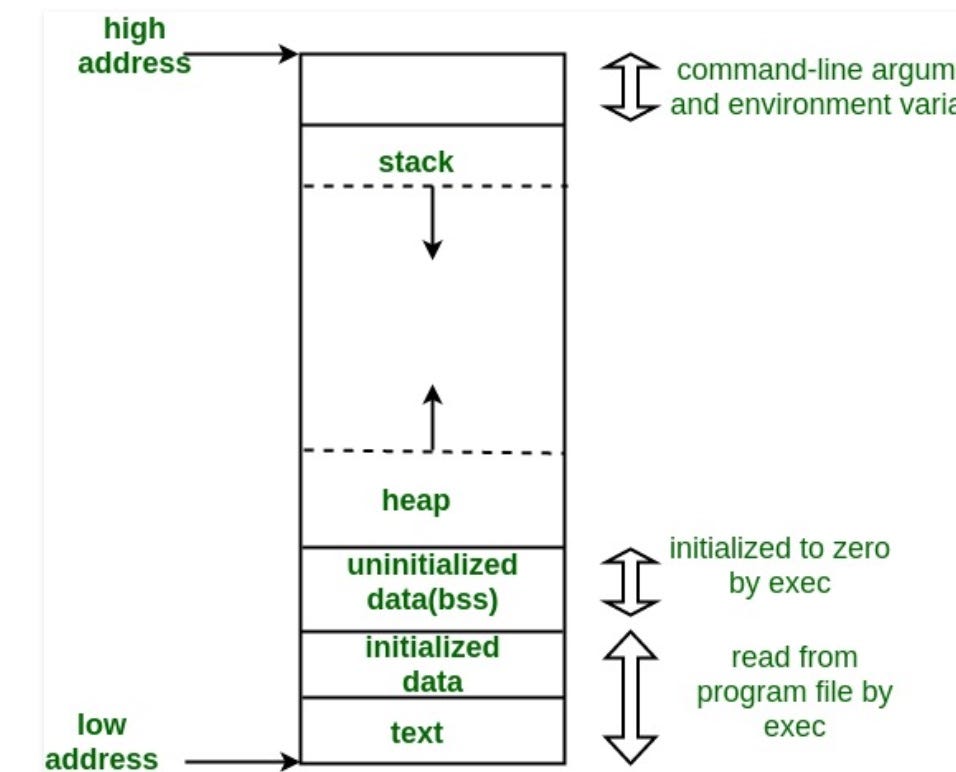
Historical context:
Early programs primarily used static structures due to limited memory and the need for predictability. As memory became more abundant and programs more complex, dynamic structures became increasingly important.
Evolution:
- Early days: Programs used mostly static arrays and structures.
- Introduction of pointers: Allowed for more flexible memory management.
- Development of dynamic allocation: Enabled the creation of data structures that could grow and shrink as needed.
- Modern era: High-level languages often abstract away the details, but understanding the underlying principles remains crucial for optimization.
Impact on programming:
- Static structures are still used for their speed and simplicity in certain scenarios.
- Dynamic structures enable more flexible and scalable programs, crucial for modern software development.
- Understanding both allows programmers to make informed decisions based on performance needs, memory constraints, and problem requirements.
In conclusion, learning about data structures, including the fundamental concepts of data storage and the distinction between static and dynamic structures, is essential for any programmer. It provides the foundation for writing efficient, scalable, and robust software, regardless of the evolution of computer hardware and programming languages.
Elementary Data Structure: The Array
Definition
An Array is a fundamental data structure that stores a fixed-size sequential collection of elements of the same type.
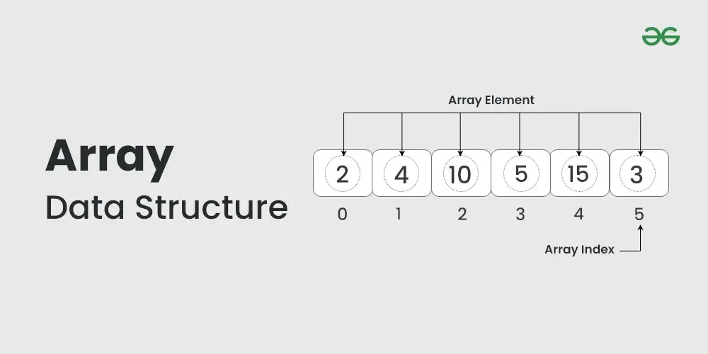
Key Properties
- Fixed Size: Once declared, the size of an array is fixed.
- Homogeneous: All elements in an array must be of the same data type.
- Contiguous Memory: Elements are stored in contiguous memory locations.
- Zero-Indexed: The first element is typically accessed with index 0 (in most programming languages).
- Random Access: Elements can be accessed directly using their index.
*Time Complexity
- Access: O(1)
- Search: O(n) for unsorted, O(log n) for sorted (using binary search)
- Insertion: O(n)
- Deletion: O(n)
Memory Usage
- Memory = (size of data type) * (number of elements)
Advantages
- Simple and easy to use
- Fast access to elements (constant time)
- Efficient for storing and accessing sequential data
Disadvantages
- Fixed size (can't be changed after declaration)
- Inefficient insertion and deletion
- Wasted memory if not all elements are used
*Common Operations
- Traversal: Visiting each element of the array
- Insertion: Adding an element at a given index
- Deletion: Removing an element from a given index
- Search: Finding the index of a given element
- Update: Modifying the value of an existing element
*Types of Arrays
- One-dimensional: Linear array (e.g.,
[1, 2, 3, 4, 5]) - Multi-dimensional (Matrices): Array of arrays (e.g., 2D array:
[[1, 2], [3, 4]])
Use Cases
- Storing and manipulating sequential data
- Implementing other data structures (e.g., stacks, queues)
- Buffering in I/O operations
- Lookup tables and hash tables
Real World Applications
Arrays are versatile data structures that can be applied to solve various real-world problems. Here are some examples:
-
Image Processing
- Representing digital images as 2D arrays of pixels
- Applying filters and transformations to images
-
Financial Applications
- Storing and analyzing time series data (e.g., stock prices over time)
- Managing portfolios and calculating returns
-
Inventory Management
- Tracking product quantities and locations in warehouses
- Managing stock levels and reordering
-
Scheduling and Calendars
- Representing days, weeks, or months in calendar applications
- Managing time slots for appointments or reservations
-
Sensor Data Collection
- Storing readings from multiple sensors over time
- Analyzing environmental data (e.g., temperature, humidity)
-
Game Development
- Representing game boards (e.g., chess, tic-tac-toe)
- Managing character inventories or attributes
-
Audio Processing
- Storing and manipulating audio samples
- Implementing digital audio effects
-
Database Systems
- Implementing index structures for faster data retrieval
- Storing and managing records in memory
-
Text Editors and Word Processors
- Storing lines of text for efficient editing and display
- Implementing undo/redo functionality
-
Network Packet Management
- Buffering and processing network packets
- Implementing network protocols
-
Scientific Computing
- Storing and manipulating matrices for linear algebra operations
- Implementing numerical methods and simulations
-
Geographic Information Systems (GIS)
- Representing map data as grids
- Storing and analyzing spatial information
-
Memory Management in Operating Systems
- Managing memory allocation and deallocation
- Implementing page tables for virtual memory
-
Compiler Design
- Storing and manipulating tokens during lexical analysis
- Managing symbol tables
-
Data Compression
- Implementing run-length encoding
- Storing frequency tables for Huffman coding
Memory Techniques for Retention
- Visualization: Imagine an array as a row of boxes, each containing a value.
- Analogy: Compare an array to building with ground floor 0.
- Acronym: FHCRZ (Fixed, Homogeneous, Contiguous, Random access, Zero-indexed)
Code Example (Python)
# Creating an array
fruits = ["apple", "banana", "cherry", "date", "elderberry"]
# Accessing elements
print(fruits[0]) # Output: apple
print(fruits[-1]) # Output: elderberry
# Updating an element
fruits[1] = "blackberry"
# Traversing the array
for fruit in fruits:
print(fruit)
# Finding the length
print(len(fruits)) # Output: 5
# Slicing
print(fruits[1:4]) # Output: ['blackberry', 'cherry', 'date']
List (Dynamic Array) Data Structure
Definition
A List, also known as a Dynamic Array, is a data structure that allows elements to be added or removed, and can grow or shrink in size automatically.
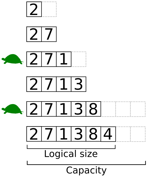
Key Properties
- Dynamic Size: Can grow or shrink as needed.
- Heterogeneous (in some languages): Can store elements of different data types (e.g., in Python).
- Contiguous Memory: Elements are stored in contiguous memory locations.
- Zero-Indexed: The first element is typically accessed with index 0 (in most programming languages).
- Random Access: Elements can be accessed directly using their index.
Time Complexity
- Access: O(1)
- Search: O(n) for unsorted, O(log n) for sorted (using binary search)
- Insertion: O(1) amortized for append, O(n) for arbitrary position
- Deletion: O(n)
Memory Usage
- Initial Memory = (size of data type) * (initial capacity)
- Grows dynamically, often doubling in size when capacity is reached
Advantages
- Flexible size (can grow or shrink as needed)
- Fast access to elements (constant time)
- Efficient for storing and accessing sequential data
- Supports various built-in operations and methods
Disadvantages
- Slower insertions and deletions compared to linked lists
- May waste some memory due to over-allocation
- Resizing operations can be costly
Common Operations
- Append: Adding an element to the end of the list
- Insert: Adding an element at a specific index
- Remove: Deleting an element by value or index
- Pop: Removing and returning the last element
- Index: Finding the position of a given element
- Slice: Extracting a portion of the list
- Sort: Arranging elements in a specific order
Implementation Details
- Resizing: When capacity is reached, a new, larger array is allocated (typically 2x size)
- Amortized Analysis: Explains O(1) average time for append operations
Use Cases
- Implementing stacks and queues
- Managing collections of data in memory
- Representing polynomials or sparse matrices
- Building more complex data structures
Memory Techniques for Retention
- Visualization: Imagine a rubber band that can stretch to accommodate more items
- Analogy: Compare a list to an accordion folder that can expand or contract
- Acronym: DCHRO (Dynamic, Contiguous, Heterogeneous, Resizable, Operations-rich)
- Chunking: Group properties into categories (e.g., structural, performance, operations)
Code Example (Python)
# Creating a list
fruits = ["apple", "banana", "cherry"]
# Appending elements
fruits.append("date")
fruits.extend(["elderberry", "fig"])
# Inserting at a specific index
fruits.insert(1, "blackberry")
# Removing elements
fruits.remove("cherry")
last_fruit = fruits.pop()
# Accessing elements
print(fruits[0]) # Output: apple
print(fruits[-1]) # Output: elderberry
# Slicing
print(fruits[1:4]) # Output: ['blackberry', 'banana', 'date']
# Sorting
fruits.sort()
print(fruits) # Output: ['apple', 'banana', 'blackberry', 'date', 'elderberry']
# List comprehension
squares = [x**2 for x in range(5)]
print(squares) # Output: [0, 1, 4, 9, 16]
Stack Data Structure
Definition
A Stack is a linear data structure that follows the Last-In-First-Out (LIFO) principle. Elements are added to and removed from the same end, called the "top" of the stack.
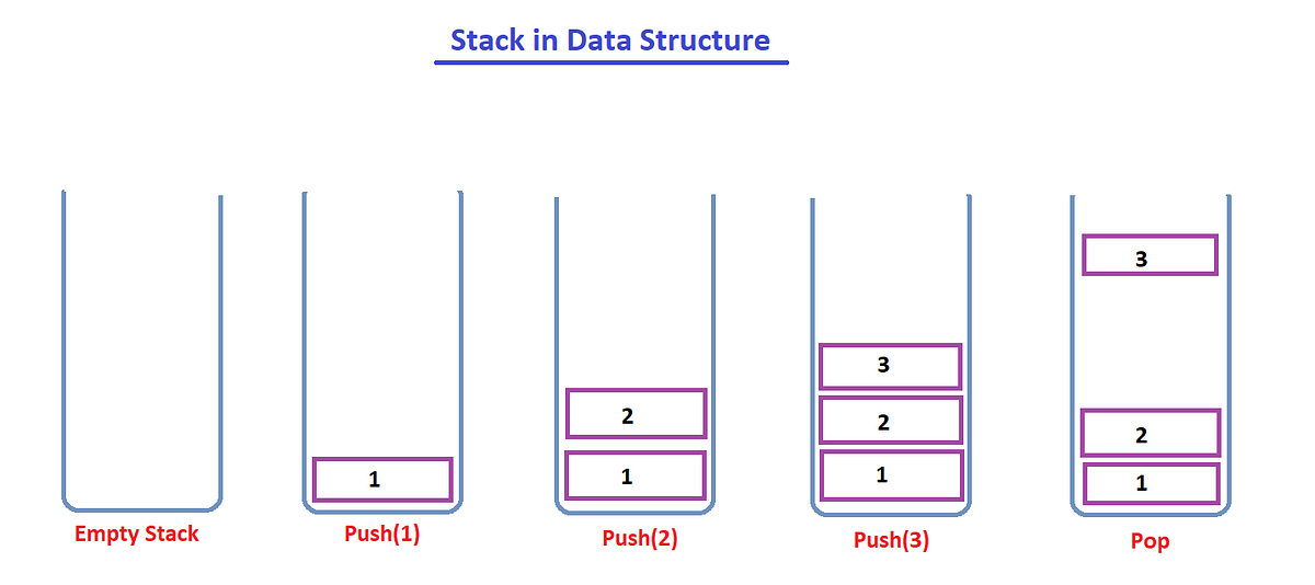
Key Properties
- LIFO (Last-In-First-Out): The last element added is the first one to be removed.
- Single-ended: Elements are added and removed only from one end (the top).
- Abstract Data Type (ADT): Can be implemented using arrays or linked lists.
- Dynamic Size: Typically grows and shrinks as elements are pushed and popped.
Basic Operations
- Push: Add an element to the top of the stack
- Pop: Remove and return the top element from the stack
- Peek/Top: View the top element without removing it
- isEmpty: Check if the stack is empty
Time Complexity
- Push: O(1)
- Pop: O(1)
- Peek: O(1)
- Search: O(n)
Memory Usage
- Depends on the underlying implementation (array-based or linked list-based)
- Memory = (size of data type) * (number of elements)
Advantages
- Simple and easy to implement
- Efficient insertion and deletion (constant time)
- Memory efficient (when implemented with a linked list)
- Useful for tracking state in algorithms
Disadvantages
- Limited access (only to the top element)
- Not suitable for certain types of data access patterns
- Potential for stack overflow if not managed properly
Common Use Cases
- Function call stack in programming languages
- Undo mechanisms in text editors
- Expression evaluation and syntax parsing
- Backtracking algorithms
- Browser history (back button functionality)
Real-World Applications of Stack Data Structure
- Web Browsing History
- Scenario: Implementing the "Back" button in web browsers.
- How Stack is Used: Each visited page URL is pushed onto a stack. When the user clicks "Back", the top URL is popped and loaded.
- Undo Functionality in Software
- Scenario: Providing undo capability in text editors, graphic design software, etc.
- How Stack is Used: Each action is pushed onto a stack. When the user requests an undo, the last action is popped and reversed.
- Function Call Management in Programming
- Scenario: Managing function calls and local variables in program execution.
- How Stack is Used: When a function is called, its context (parameters, local variables, return address) is pushed onto the call stack. When the function returns, its context is popped.
- Expression Evaluation in Calculators
- Scenario: Evaluating mathematical expressions, especially those with parentheses.
- How Stack is Used: Operators and operands are pushed and popped from the stack to handle operator precedence and nested expressions.
- Backtracking Algorithms
- Scenario: Solving mazes, puzzles, or in game AI for chess.
- How Stack is Used: Possible moves or states are pushed onto the stack. If a path leads to a dead-end, the program backtracks by popping the stack.
- Syntax Parsing in Compilers
- Scenario: Checking for balanced parentheses or brackets in code.
- How Stack is Used: Opening brackets are pushed onto the stack. Each closing bracket is matched with the top of the stack.
- Memory Management
- Scenario: Managing memory allocation in operating systems.
- How Stack is Used: Memory blocks are allocated and deallocated in a LIFO manner for efficient memory management.
- Recursion Simulation
- Scenario: Implementing or optimizing recursive algorithms.
- How Stack is Used: Instead of using actual recursion, which can lead to stack overflow, an explicit stack can be used to simulate recursive calls.
- Graph Algorithms
- Scenario: Depth-First Search (DFS) in graph traversal.
- How Stack is Used: Vertices to be visited are pushed onto the stack. The algorithm pops a vertex, processes it, and pushes its unvisited neighbors.
- Clipboard History
- Scenario: Maintaining a history of copied items in an operating system.
- How Stack is Used: Each copied item is pushed onto a stack. Users can cycle through previous copies by popping from the stack.
- Call Center Systems
- Scenario: Managing customer service calls in a Last-In-First-Out manner.
- How Stack is Used: Incoming calls are pushed onto a stack. The most recent caller is served first (popped) when an agent becomes available.
- Plate Stacking in Restaurants
- Scenario: Managing a stack of plates in a cafeteria or buffet.
- How Stack is Used: Clean plates are pushed onto the stack. Diners take plates from the top (pop operation).
Variations
- Min Stack: Keeps track of the minimum element
- Max Stack: Keeps track of the maximum element
- Double-ended Stack: Allows push and pop from both ends
Implementation Approaches
- Array-based: Uses a dynamic array to store elements
- Linked List-based: Uses a singly linked list with head as top
Memory Techniques for Retention
- Visualization: Imagine a stack of plates where you can only add or remove from the top
- Analogy: Compare to a Pringles can - you can only add or remove chips from the top
- Acronym: LIPS (Last-In, Push-Pop Stack)
- Mnemonic: "Last to arrive, first to leave" (like at a party)
Code Example (Python)
class Stack:
def __init__(self):
self.items = []
def is_empty(self):
return len(self.items) == 0
def push(self, item):
self.items.append(item)
def pop(self):
if not self.is_empty():
return self.items.pop()
else:
raise IndexError("Stack is empty")
def peek(self):
if not self.is_empty():
return self.items[-1]
else:
raise IndexError("Stack is empty")
def size(self):
return len(self.items)
# Usage example
stack = Stack()
stack.push(1)
stack.push(2)
stack.push(3)
print(stack.pop()) # Output: 3
print(stack.peek()) # Output: 2
print(stack.size()) # Output: 2
Queue Data Structure
Definition
A Queue is a linear data structure that follows the First-In-First-Out (FIFO) principle. Elements are added at one end (rear) and removed from the other end (front).
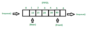
Key Properties
- FIFO (First-In-First-Out): The first element added is the first one to be removed.
- Two-ended: Elements are added at the rear and removed from the front.
- Abstract Data Type (ADT): Can be implemented using arrays or linked lists.
- Dynamic Size: Typically grows and shrinks as elements are enqueued and dequeued.
Basic Operations
- Enqueue: Add an element to the rear of the queue
- Dequeue: Remove and return the front element from the queue
- Front: View the front element without removing it
- isEmpty: Check if the queue is empty
- Size: Get the number of elements in the queue
Time Complexity
- Enqueue: O(1)
- Dequeue: O(1)
- Front: O(1)
- isEmpty: O(1)
- Size: O(1)
Memory Usage
- Depends on the underlying implementation (array-based or linked list-based)
- Memory = (size of data type) * (number of elements)
Advantages
- Maintains order of insertion
- Efficient insertion and deletion (constant time)
- Useful for managing resources and scheduling
- Supports both synchronous and asynchronous processing
Disadvantages
- Fixed size in array-based implementation (can be mitigated with circular queue)
- Potential for queue overflow or underflow if not managed properly
- No random access to elements
Common Use Cases
- Task scheduling in operating systems
- Breadth-First Search algorithm in graphs
- Print job spooling
- Handling of requests on a single shared resource (e.g., CPU)
- Buffering for data streams
Real World Application
Queues are widely used in computer science and everyday life to manage processes where first-come, first-served order is important. Here are some practical applications:
- Customer Service Systems
- Call Centers: Incoming calls are placed in a queue and answered in the order they were received.
- Help Desk Ticketing: Support requests are processed in the order they are submitted.
- Transportation and Logistics
- Traffic Management: Vehicles at a traffic signal are served in the order they arrive.
- Airline Boarding: Passengers board the plane based on their order in the queue.
- Shipping and Delivery: Orders are processed and shipped based on their order in the queue.
- Operating Systems
- CPU Scheduling: Processes waiting for CPU time are managed in a queue.
- Print Spooling: Print jobs are processed in the order they are received.
- I/O Buffer Management: Data is read from or written to devices in a queued order.
- Networking
- Routers and Switches: Network packets are queued before being transmitted.
- Web Servers: HTTP requests are often processed in a FIFO manner.
- Healthcare
- Emergency Room Triage: While not strictly FIFO due to severity considerations, queues help manage patient wait times.
- Organ Donation Lists: Patients waiting for organ transplants are often managed in a queue-like system.
- Entertainment and Services
- Ticket Sales: Online queuing systems for high-demand event tickets.
- Amusement Park Ride Lines: Physical queues for managing ride access.
- Streaming Services: Video or audio buffers use queues to ensure smooth playback.
- Manufacturing and Production
- Assembly Lines: Products move through stages of assembly in a queue-like manner.
- Inventory Management: First-In-First-Out (FIFO) method for perishable goods.
- Software and Web Development
- Task Scheduling: Background jobs or tasks are often managed in queues.
- Message Brokers: Systems like RabbitMQ use queues to manage message passing between services.
- Financial Systems
- Transaction Processing: Banking transactions are often processed in the order they are received.
- Stock Market Orders: Some types of stock market orders are processed in a FIFO manner.
- Education
- Course Waitlists: Students are added to course waitlists in the order they apply.
- Grading Systems: Some professors grade assignments in the order they were submitted.
Variations
- Circular Queue: Efficient use of fixed-size array
- Double-ended Queue (Deque): Allows insertion and deletion at both ends
- Priority Queue: Elements have associated priorities
Implementation Approaches
- Array-based: Uses a dynamic or circular array to store elements
- Linked List-based: Uses a singly linked list with front and rear pointers
Memory Techniques for Retention
- Visualization: Imagine a line of people waiting for a bus - first in line is first to board
- Analogy: Compare to a pipe where items enter one end and exit the other
- Acronym: FIFE (First-In, First-Exit)
- Mnemonic: "First to arrive, first to leave" (like at a bakery)
Code Example (Python)
from collections import deque
class Queue:
def __init__(self):
self.items = deque()
def is_empty(self):
return len(self.items) == 0
def enqueue(self, item):
self.items.append(item)
def dequeue(self):
if not self.is_empty():
return self.items.popleft()
else:
raise IndexError("Queue is empty")
def front(self):
if not self.is_empty():
return self.items[0]
else:
raise IndexError("Queue is empty")
def size(self):
return len(self.items)
# Usage example
queue = Queue()
queue.enqueue("Task 1")
queue.enqueue("Task 2")
queue.enqueue("Task 3")
print(queue.dequeue()) # Output: Task 1
print(queue.front()) # Output: Task 2
print(queue.size()) # Output: 2
Remember: Implement and experiment with queues in your preferred programming language to reinforce your understanding!
Deque (Double-ended Queue) Data Structure
Definition
A Deque (pronounced "deck") is a linear data structure that allows insertion and deletion of elements from both ends. It combines the features of both stacks and queues.
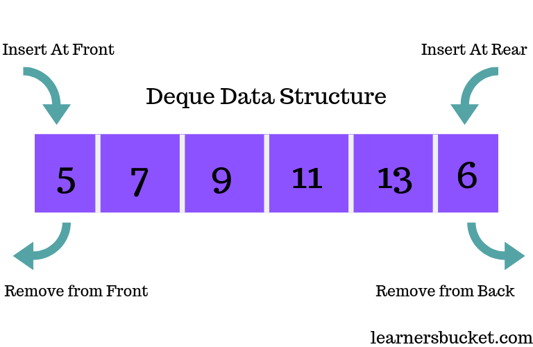
Key Properties
- Double-ended: Elements can be added or removed from both front and rear.
- Flexible: Supports both LIFO (Last-In-First-Out) and FIFO (First-In-First-Out) operations.
- Abstract Data Type (ADT): Can be implemented using dynamic arrays or doubly linked lists.
- Dynamic Size: Typically grows and shrinks as elements are added and removed.
Basic Operations
- insertFront: Add an element to the front of the deque
- insertRear: Add an element to the rear of the deque
- deleteFront: Remove and return the front element
- deleteRear: Remove and return the rear element
- getFront: View the front element without removing it
- getRear: View the rear element without removing it
- isEmpty: Check if the deque is empty
- size: Get the number of elements in the deque
Time Complexity
- All basic operations (insertFront, insertRear, deleteFront, deleteRear, getFront, getRear): O(1)
- isEmpty: O(1)
- size: O(1)
Memory Usage
- Depends on the underlying implementation (array-based or linked list-based)
- Memory = (size of data type) * (number of elements) + overhead for pointers (in linked list implementation)
Advantages
- Combines functionality of both stacks and queues
- Efficient insertion and deletion at both ends (constant time)
- Flexible for various use cases
- Supports both LIFO and FIFO operations
Disadvantages
- More complex implementation compared to simple stacks or queues
- Slightly higher memory usage due to additional pointers (in linked list implementation)
- No random access to elements (except in array-based implementations)
Common Use Cases
- Implementing undo-redo functionality
- Managing work stealing in multiprocessing environments
- Palindrome checking
- Sliding window problems in algorithms
- Browser history (forward and backward navigation)
Real-World Use Cases for Deques (Double-ended Queues)
- Undo-Redo Functionality in Applications
- Scenario: Text editors, graphic design software, or any application with undo-redo features.
- Solution: Use a deque to store user actions. Recent actions are added to one end for undo, and when undone, they're moved to the other end for potential redo.
- Benefit: Efficient O(1) operations for both undo and redo actions.
- Browser History Navigation
- Scenario: Implementing forward and backward navigation in web browsers.
- Solution: Use a deque to store visited web pages. The current page is at one end, previously visited pages at the other. New pages are added to the front, and navigation uses both ends.
- Benefit: Quick access to both recently visited and older pages.
- Task Scheduling in Operating Systems
- Scenario: Managing processes or tasks in a multi-tasking environment.
- Solution: Use a deque for task queues. High-priority tasks can be added to the front, while regular tasks are added to the rear.
- Benefit: Flexible prioritization of tasks without separate data structures.
- Palindrome Checking
- Scenario: Efficiently checking if a word or phrase is a palindrome.
- Solution: Use a deque to store characters. Compare characters from both ends, moving inwards.
- Benefit: O(n/2) comparisons, with easy handling of even and odd-length strings.
- Sliding Window Problems in Data Analysis
- Scenario: Analyzing time series data or streaming data with a fixed-size window.
- Solution: Use a deque to represent the sliding window. Add new elements to one end and remove old elements from the other.
- Benefit: Efficient updates to the window contents as it slides over the data.
- A-Steal Work Scheduling Algorithm
- Scenario: Load balancing in parallel computing environments.
- Solution: Each processor maintains a deque of tasks. Busy processors add tasks to one end, while idle processors can steal tasks from the other end of busy processors' deques.
- Benefit: Efficient work distribution and load balancing.
- Network Packet Processing
- Scenario: Managing network packets in routers or switches.
- Solution: Use deques to handle packet queues. High-priority packets can be inserted at the front, while normal packets are added to the rear.
- Benefit: Flexible packet prioritization and efficient processing.
- Music Player Playlist Management
- Scenario: Implementing features like "play next" and "add to queue" in music players.
- Solution: Use a deque to manage the playlist. New songs can be added to either the front ("play next") or the back ("add to queue").
- Benefit: Flexible playlist management with efficient insertions at both ends.
- Customer Service Queue Management
- Scenario: Managing customer service requests with priority handling.
- Solution: Use a deque for the customer queue. VIP customers can be added to the front, while regular customers join at the rear.
- Benefit: Efficient prioritization without multiple separate queues.
- Memory-Efficient Caching
- Scenario: Implementing a cache with both FIFO and LIFO eviction policies.
- Solution: Use a deque to store cached items. New items can be added to one end, and eviction can happen from either end based on the desired policy.
- Benefit: Flexible caching strategy with efficient insertions and deletions.
Remember: The key advantage of deques in these scenarios is their ability to efficiently handle operations at both ends, providing flexibility that single-ended data structures like stacks or queues cannot match.
Variations
- Scroll Buffer: Used in text editors for efficient insertion and deletion
- A-Steal Deque: Used in work-stealing schedulers
Implementation Approaches
- Array-based: Uses a dynamic circular array
- Linked List-based: Uses a doubly linked list
Memory Techniques for Retention
- Visualization: Imagine a double-ended subway train where passengers can board and exit from both ends
- Analogy: Compare to a deck of cards where you can add or remove cards from both top and bottom
- Acronym: DIDO (Double-In, Double-Out)
- Mnemonic: "First or last, in or out, deque handles it all about"
Code Example (Python)
from collections import deque
class Deque:
def __init__(self):
self.items = deque()
def is_empty(self):
return len(self.items) == 0
def insert_front(self, item):
self.items.appendleft(item)
def insert_rear(self, item):
self.items.append(item)
def delete_front(self):
if not self.is_empty():
return self.items.popleft()
else:
raise IndexError("Deque is empty")
def delete_rear(self):
if not self.is_empty():
return self.items.pop()
else:
raise IndexError("Deque is empty")
def get_front(self):
if not self.is_empty():
return self.items[0]
else:
raise IndexError("Deque is empty")
def get_rear(self):
if not self.is_empty():
return self.items[-1]
else:
raise IndexError("Deque is empty")
def size(self):
return len(self.items)
# Usage example
deque = Deque()
deque.insert_front("A")
deque.insert_rear("B")
deque.insert_front("C")
print(deque.delete_front()) # Output: C
print(deque.delete_rear()) # Output: B
print(deque.get_front()) # Output: A
print(deque.size()) # Output: 1
Linked List Data Structure
Definition
A Linked List is a linear data structure where elements are stored in nodes. Each node contains a data field and a reference (or link) to the next node in the sequence.

Key Properties
- Dynamic Size: Can grow or shrink in size during execution.
- Non-contiguous Memory: Nodes can be stored anywhere in memory.
- Efficient Insertion/Deletion: Adding or removing elements doesn't require shifting other elements.
- Sequential Access: Elements are accessed sequentially starting from the first node.
Types of Linked Lists
- Singly Linked List: Each node points to the next node.
- Doubly Linked List: Each node has pointers to both next and previous nodes.
- Circular Linked List: Last node points back to the first node.
Basic Components
- Node: Contains data and pointer(s) to other node(s).
- Head: Points to the first node in the list.
- Tail: Points to the last node in the list (in some implementations).
Basic Operations
- Insertion: Add a new node (at the beginning, end, or middle).
- Deletion: Remove a node (from the beginning, end, or middle).
- Traversal: Visit each node in the list.
- Search: Find a node with a specific value.
Time Complexity
- Access: O(n)
- Search: O(n)
- Insertion: O(1) if inserting at known position, O(n) if searching first
- Deletion: O(1) if deleting known position, O(n) if searching first
Memory Usage
- Memory = (size of data + size of pointer) * (number of nodes)
- Additional memory for head (and tail) pointers
Advantages
- Dynamic size
- Efficient insertions and deletions
- No memory wastage (allocates exact memory required)
- Implementation of other data structures (stacks, queues, etc.)
Disadvantages
- Sequential access (no random access)
- Extra memory for pointers
- Not cache-friendly due to non-contiguous memory allocation
Common Use Cases
- Implementation of stacks, queues, and graphs
- Undo functionality in applications
- Hash tables (chaining for collision resolution)
- Polynomial arithmetic
- Music playlists
Real-World Applications of Linked Lists
Linked Lists are versatile data structures that find applications in various real-world scenarios. Here are some practical situations where Linked Lists are commonly used:
- Music Player Playlists
- Scenario: Managing a list of songs in a music player.
- Application: Each node represents a song, containing metadata and a pointer to the next song.
- Benefit: Easy to add, remove, or reorder songs without affecting the entire playlist.
- Browser History
- Scenario: Implementing forward and backward navigation in web browsers.
- Application: Each node represents a webpage, with links to both previous and next pages (doubly linked list).
- Benefit: Efficient navigation through browser history in both directions.
- Image Viewer Carousel
- Scenario: Creating a circular image gallery or slideshow.
- Application: Each node contains an image, with the last image linking back to the first (circular linked list).
- Benefit: Smooth, continuous navigation through images in both directions.
- Undo Functionality in Text Editors
- Scenario: Implementing undo/redo features in word processors or text editors.
- Application: Each node represents a state of the document, allowing easy traversal through edit history.
- Benefit: Efficient storage and navigation of document states for undo/redo operations.
- Memory Management in Operating Systems
- Scenario: Managing free memory blocks in an operating system.
- Application: Each node represents a free memory block, easily split or merged as needed.
- Benefit: Efficient allocation and deallocation of memory without fragmentation.
- Job Queue in Print Spoolers
- Scenario: Managing print jobs in a printer queue.
- Application: Each node represents a print job, easily added or removed from the queue.
- Benefit: Flexible management of print jobs, allowing priority insertions or cancellations.
- Polynomial Arithmetic
- Scenario: Representing and manipulating polynomials in mathematical software.
- Application: Each node represents a term in the polynomial, with easy insertion and removal of terms.
- Benefit: Efficient storage and manipulation of polynomials with varying numbers of terms.
- Card Games
- Scenario: Implementing a deck of cards in digital card games.
- Application: Each node represents a card, allowing easy shuffling, dealing, and returning to the deck.
- Benefit: Flexible manipulation of the deck without need for shifting elements.
- Symbol Tables in Compilers
- Scenario: Managing symbols (variables, functions) during compilation.
- Application: Each node represents a symbol, with easy insertion, deletion, and lookup.
- Benefit: Efficient management of symbols with varying lifetimes during compilation.
- Social Media Feed
- Scenario: Implementing an infinite scroll feature in social media apps.
- Application: Each node represents a post, with new posts easily added to the top or bottom of the feed.
- Benefit: Efficient insertion of new content and removal of old content in the feed.
Remember: These applications leverage the key strengths of Linked Lists, such as dynamic size, efficient insertions and deletions, and flexible memory allocation. Understanding these real-world use cases can provide valuable context for when to consider using Linked Lists in your own projects.
Variations
- Skip List: Multiple layers of linked lists for faster searching
- Unrolled Linked List: Storing multiple elements in each node
- XOR Linked List: Memory-efficient doubly linked list using bitwise XOR
Memory Techniques for Retention
- Visualization: Imagine a train where each car (node) is connected to the next by a coupling (pointer).
- Analogy: Compare to a scavenger hunt where each clue points to the location of the next clue.
- Acronym: LEND (Linked Elements with Node Data)
- Mnemonic: "Link by link, the chain grows long, each points ahead, where it belongs"
Code Example (Python)
class Node:
def __init__(self, data):
self.data = data
self.next = None
class LinkedList:
def __init__(self):
self.head = None
def is_empty(self):
return self.head is None
def insert_front(self, data):
new_node = Node(data)
new_node.next = self.head
self.head = new_node
def insert_end(self, data):
new_node = Node(data)
if self.is_empty():
self.head = new_node
else:
current = self.head
while current.next:
current = current.next
current.next = new_node
def delete_front(self):
if not self.is_empty():
self.head = self.head.next
else:
raise IndexError("List is empty")
def search(self, data):
current = self.head
while current:
if current.data == data:
return True
current = current.next
return False
def display(self):
elements = []
current = self.head
while current:
elements.append(current.data)
current = current.next
return ' -> '.join(map(str, elements))
# Usage example
ll = LinkedList()
ll.insert_end(1)
ll.insert_end(2)
ll.insert_front(0)
print(ll.display()) # Output: 0 -> 1 -> 2
print(ll.search(1)) # Output: True
ll.delete_front()
print(ll.display()) # Output: 1 -> 2
Doubly Linked List Data Structure
Definition
A Doubly Linked List is a linear data structure where each node contains data and two references (or links): one to the next node and one to the previous node in the sequence.
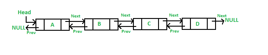
Key Properties
- Bidirectional: Can be traversed in both forward and backward directions.
- Dynamic Size: Can grow or shrink in size during execution.
- Non-contiguous Memory: Nodes can be stored anywhere in memory.
- Efficient Insertion/Deletion: Adding or removing elements is O(1) when position is known.
Basic Components
- Node: Contains data, a pointer to the next node, and a pointer to the previous node.
- Head: Points to the first node in the list.
- Tail: Points to the last node in the list.
Basic Operations
- Insertion: Add a new node (at the beginning, end, or middle).
- Deletion: Remove a node (from the beginning, end, or middle).
- Forward Traversal: Visit each node from head to tail.
- Backward Traversal: Visit each node from tail to head.
- Search: Find a node with a specific value.
Time Complexity
- Access: O(n)
- Search: O(n)
- Insertion: O(1) if inserting at known position, O(n) if searching first
- Deletion: O(1) if deleting known position, O(n) if searching first
Memory Usage
- Memory = (size of data + size of two pointers) * (number of nodes)
- Additional memory for head and tail pointers
Advantages
- Bidirectional traversal
- Efficient insertions and deletions at both ends
- Easy implementation of certain algorithms (e.g., LRU cache)
- Simpler to reverse the list compared to singly linked list
Disadvantages
- More memory usage due to extra pointer
- Slightly more complex implementation than singly linked list
- Still no random access
- Potential for inconsistency if pointers are not updated correctly
Common Use Cases
- Implementation of advanced data structures (e.g., deques)
- Browser's forward and backward navigation
- Undo and redo functionality in applications
- Music player (next and previous track)
- Implementing LRU (Least Recently Used) cache
Real-World Use Cases of Doubly Linked Lists
Doubly Linked Lists find applications in various real-world scenarios due to their unique properties, particularly their ability to traverse in both directions and efficiently insert or delete elements at any position. Here are some prominent use cases:
-
Browser History Navigation
- Implementing the back and forward functionality in web browsers.
- Each node represents a webpage, allowing quick navigation in both directions.
-
Music Player Playlists
- Managing playlists where users can move both forward and backward through tracks.
- Efficient for adding or removing songs from any position in the playlist.
-
Undo-Redo Functionality
- In text editors, graphic design software, or any application with undo-redo features.
- Each node represents a state, allowing easy navigation through edit history.
-
Cache Management (e.g., LRU Cache)
- Implementing Least Recently Used (LRU) cache, where both ends of the list need to be accessed quickly.
- Efficient for moving recently used items to the front and removing least used items from the end.
-
Image Viewer Applications
- Allowing users to scroll through images in both directions.
- Efficient for loading next/previous images and maintaining a viewing history.
-
Text Editors with Cursor Movement
- Implementing efficient cursor movement in both directions in text editors.
- Facilitates operations like insert, delete, and navigate through text.
-
Palindrome Checking
- Efficient algorithm for checking if a long string or linked list is a palindrome.
- Can traverse from both ends towards the middle simultaneously.
-
Train Carriage Management Systems
- Modeling train compositions where carriages can be added or removed from either end.
- Useful for efficiently reorganizing carriages.
-
Multi-level Undo in CAD Software
- Computer-Aided Design (CAD) software often requires complex undo-redo functionality.
- Doubly linked lists can manage multiple levels of undo and redo operations.
-
Blockchain Implementation
- In some blockchain designs, where each block needs to reference both the previous and next blocks.
- Allows for efficient verification and traversal of the blockchain in both directions.
-
Memory Management in Operating Systems
- Managing free and allocated memory blocks.
- Efficient for splitting and merging memory blocks as needed.
-
Implementation of Advanced Data Structures
- Used as a building block for more complex data structures like:
- Deques (double-ended queues)
- Circular buffers with efficient wraparound
- Specialized graph representations
- Used as a building block for more complex data structures like:
-
DNA Sequence Analysis
- Representing DNA sequences for efficient forward and backward analysis.
- Useful in bioinformatics algorithms that require bidirectional traversal of genetic data.
-
Elevator Systems
- Managing elevator requests and optimizing elevator movement.
- Efficient for handling requests in both up and down directions.
These use cases leverage the doubly linked list's ability to efficiently insert, delete, and traverse in both directions, making it a versatile data structure for scenarios requiring bidirectional access or manipulation of sequential data.
Variations
- Circular Doubly Linked List: Last node's next points to first, first node's previous points to last
- XOR Linked List: Memory-efficient version using bitwise XOR of addresses
Memory Techniques for Retention
- Visualization: Imagine a two-way street where you can move in both directions.
- Analogy: Compare to a railway train where each car is connected to both the car in front and behind.
- Acronym: BOND (Bidirectional Ordered Node Data)
- Mnemonic: "Double the links, double the direction, forward and back without objection"
Code Example (Python)
class Node:
def __init__(self, data):
self.data = data
self.next = None
self.prev = None
class DoublyLinkedList:
def __init__(self):
self.head = None
self.tail = None
def is_empty(self):
return self.head is None
def insert_front(self, data):
new_node = Node(data)
if self.is_empty():
self.head = self.tail = new_node
else:
new_node.next = self.head
self.head.prev = new_node
self.head = new_node
def insert_end(self, data):
new_node = Node(data)
if self.is_empty():
self.head = self.tail = new_node
else:
new_node.prev = self.tail
self.tail.next = new_node
self.tail = new_node
def delete_front(self):
if not self.is_empty():
if self.head == self.tail:
self.head = self.tail = None
else:
self.head = self.head.next
self.head.prev = None
else:
raise IndexError("List is empty")
def delete_end(self):
if not self.is_empty():
if self.head == self.tail:
self.head = self.tail = None
else:
self.tail = self.tail.prev
self.tail.next = None
else:
raise IndexError("List is empty")
def display_forward(self):
elements = []
current = self.head
while current:
elements.append(current.data)
current = current.next
return ' <-> '.join(map(str, elements))
def display_backward(self):
elements = []
current = self.tail
while current:
elements.append(current.data)
current = current.prev
return ' <-> '.join(map(str, elements))
# Usage example
dll = DoublyLinkedList()
dll.insert_end(1)
dll.insert_end(2)
dll.insert_front(0)
print(dll.display_forward()) # Output: 0 <-> 1 <-> 2
print(dll.display_backward()) # Output: 2 <-> 1 <-> 0
dll.delete_front()
dll.delete_end()
print(dll.display_forward()) # Output: 1
Circular Linked List Data Structure
Definition
A Circular Linked List is a variation of linked list in which the last node points back to the first node, creating a circle-like structure.
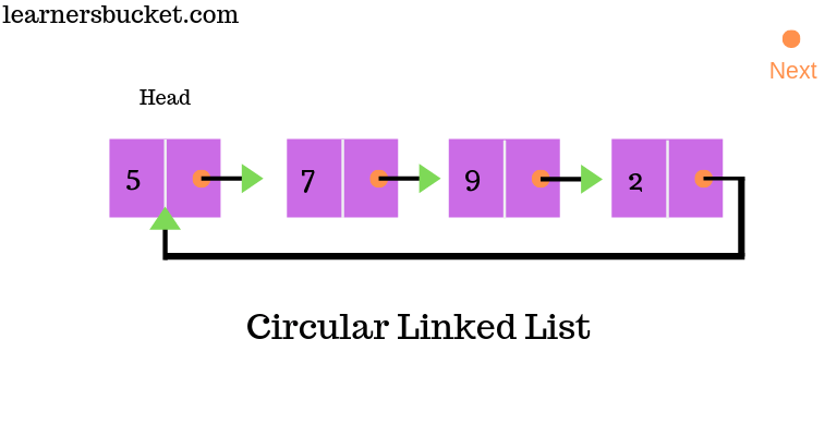
Key Properties
- Circular Structure: The last node points to the first node, forming a closed loop.
- No Null Termination: There's no null at the end of the list.
- Dynamic Size: Can grow or shrink in size during execution.
- Continuous Traversal: Can be traversed starting from any point in the list.
Types of Circular Linked Lists
- Singly Circular Linked List: Each node has a single pointer to the next node.
- Doubly Circular Linked List: Each node has pointers to both next and previous nodes.
Basic Components
- Node: Contains data and pointer(s) to other node(s).
- Head: Points to any node in the list (often the first inserted node).
Basic Operations
- Insertion: Add a new node (at the beginning, end, or middle).
- Deletion: Remove a node (from the beginning, end, or middle).
- Traversal: Visit each node in the list.
- Search: Find a node with a specific value.
Time Complexity
- Access: O(n)
- Search: O(n)
- Insertion: O(1) if inserting at known position, O(n) if searching first
- Deletion: O(1) if deleting known position, O(n) if searching first
Memory Usage
- Memory = (size of data + size of pointer) * (number of nodes)
- No additional memory for tail pointer needed
Advantages
- Constant-time insertion at the beginning and end of the list
- Simplified list operations (no need to check for null)
- Useful for applications that require repetitive cycling through a list
- Efficient memory utilization (no null pointers)
Real-World Use Cases of Circular Linked Lists
Circular Linked Lists find applications in various domains due to their unique properties. Here are some notable real-world use cases:
-
Operating System Resource Management
- Process Scheduling: Used in round-robin scheduling algorithms where each process gets a fixed time slice in a cyclic manner.
- Memory Management: In systems using circular memory allocation strategies.
-
Computer Networking
- Token Ring Networks: In this network topology, a token is passed around the network in a circular manner.
- Bluetooth Device Discovery: For managing the list of discoverable devices in a circular fashion.
-
Multimedia Applications
- Playlist Management: For creating looping playlists in music or video players.
- Image Carousel: In web and mobile applications for cycling through images.
-
Gaming
- Turn-Based Board Games: To manage player turns in multiplayer games.
- Circular Buffering in Game Engines: For efficient memory management in game loops.
-
Embedded Systems
- Task Scheduling: In real-time operating systems for cyclic execution of tasks.
- Circular Buffers: Used in data logging and communication protocols.
-
Database Systems
- Query Optimization: For managing circular dependencies in query execution plans.
- Buffer Pool Management: In database management systems for cyclical page replacement.
-
Computer Graphics
- Vertex Management: In 3D graphics for closed polygonal models.
- Animation Loops: For creating seamless looping animations.
-
Timekeeping and Scheduling Applications
- Circular Clock Representations: For digital clock implementations.
- Appointment Scheduling: In calendar applications for recurring events.
-
Text Editing and Word Processing
- Undo-Redo Functionality: Maintaining a circular history of document changes.
- Cursor Movement: For wrapping cursor movement in text editors.
-
Financial Systems
- Rotating Savings and Credit Associations (ROSCAs): For managing cyclical distribution of funds.
- Circular Debt Management: In financial modeling of circular debt scenarios.
-
Transportation and Logistics
- Traffic Light Control Systems: For cyclic management of traffic signal phases.
- Delivery Route Optimization: In logistics for routes that return to the starting point.
-
Telecommunications
- Call Center Queue Management: For fair distribution of incoming calls to agents.
- Cellular Network Channel Allocation: In mobile networks for frequency reuse patterns.
-
Manufacturing and Industrial Automation
- Assembly Line Management: For cyclical process control in manufacturing.
- Robotic Arm Movement: In industrial robots for repetitive task execution.
-
Scientific Simulations
- Planetary Orbit Calculations: In astrophysics simulations.
- Molecular Structure Modeling: For cyclic molecular structures in chemistry.
These use cases demonstrate the versatility of Circular Linked Lists in solving problems that involve cyclic or repetitive processes, resource sharing, and efficient memory management across various fields and industries.
Disadvantages
- Slightly more complex implementation than singly linked list
- Risk of infinite loops if not implemented carefully
- No natural end point, requiring special consideration during traversal
Common Use Cases
- Round-robin scheduling in operating systems
- Implementing circular buffers
- Managing computer resources in a multi-user environment
- Multiplayer board games (turn rotation)
- Repetitive task management in embedded systems
Variations
- Josephus Problem: A counting-out game, often implemented using circular linked lists
- Circular Buffer: Also known as a ring buffer, used in embedded systems and data streaming
Memory Techniques for Retention
- Visualization: Imagine a merry-go-round where you can start from any horse and go around indefinitely.
- Analogy: Compare to a circular race track where runners keep going around without a finish line.
- Acronym: CIRCLE (Circularly Interconnected Repeating Cyclic Linked Elements)
- Mnemonic: "Round and round the list we go, where it stops, there's no null to show"
Code Example (Python)
class Node:
def __init__(self, data):
self.data = data
self.next = None
class CircularLinkedList:
def __init__(self):
self.head = None
def is_empty(self):
return self.head is None
def insert_end(self, data):
new_node = Node(data)
if self.is_empty():
self.head = new_node
new_node.next = self.head
else:
current = self.head
while current.next != self.head:
current = current.next
current.next = new_node
new_node.next = self.head
def insert_beginning(self, data):
new_node = Node(data)
if self.is_empty():
self.head = new_node
new_node.next = self.head
else:
current = self.head
while current.next != self.head:
current = current.next
new_node.next = self.head
current.next = new_node
self.head = new_node
def delete(self, key):
if self.is_empty():
return
if self.head.data == key and self.head.next == self.head:
self.head = None
elif self.head.data == key:
current = self.head
while current.next != self.head:
current = current.next
current.next = self.head.next
self.head = self.head.next
else:
current = self.head
prev = None
while current.next != self.head:
prev = current
current = current.next
if current.data == key:
prev.next = current.next
break
def display(self):
if self.is_empty():
return "List is empty"
elements = []
current = self.head
while True:
elements.append(str(current.data))
current = current.next
if current == self.head:
break
return ' -> '.join(elements) + ' -> (back to start)'
# Usage example
cll = CircularLinkedList()
cll.insert_end(1)
cll.insert_end(2)
cll.insert_beginning(0)
print(cll.display()) # Output: 0 -> 1 -> 2 -> (back to start)
cll.delete(1)
print(cll.display()) # Output: 0 -> 2 -> (back to start)
Tree Data Structure
Definition
A Tree is a hierarchical data structure consisting of nodes connected by edges. It starts with a root node and branches out to child nodes, forming a parent-child relationship between nodes.
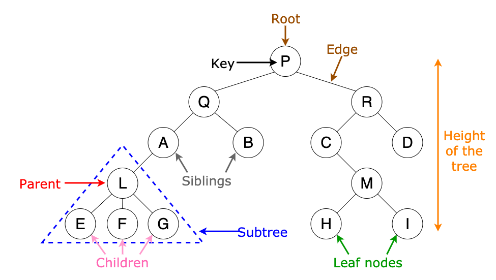
Key Properties
- Hierarchical Structure: Organizes data in a parent-child relationship.
- Root Node: The topmost node of the tree.
- Parent and Child Nodes: Each node (except the root) has one parent and can have multiple children.
- Leaf Nodes: Nodes with no children.
- Subtree: A tree structure formed by a node and its descendants.
- Depth: The number of edges from the root to a node.
- Height: The number of edges on the longest path from a node to a leaf.
Types of Trees
- Binary Tree: Each node has at most two children.
- Binary Search Tree (BST): A binary tree with ordered nodes.
- AVL Tree: Self-balancing binary search tree.
- Red-Black Tree: Self-balancing binary search tree with color properties.
- N-ary Tree: Each node can have N children.
- Trie: Used for storing strings, where each node represents a character.
Basic Components
- Node: Contains data and references to its children.
- Root: The topmost node of the tree.
- Edge: The link between two nodes.
Basic Operations
- Insertion: Add a new node to the tree.
- Deletion: Remove a node from the tree.
- Traversal: Visit all nodes of the tree (In-order, Pre-order, Post-order, Level-order).
- Search: Find a node with a specific value.
Time Complexity (for balanced binary trees)
- Access: O(log n)
- Search: O(log n)
- Insertion: O(log n)
- Deletion: O(log n)
Memory Usage
- Memory = (size of data + size of pointers to children) * (number of nodes)
Advantages
- Hierarchical data representation
- Efficient searching and sorting (in balanced trees)
- Natural representation for recursive structures
- Basis for many advanced data structures and algorithms
Disadvantages
- Can become unbalanced, leading to poor performance
- More complex to implement than linear data structures
- May require more memory due to pointer overhead
Common Use Cases
- File systems in operating systems
- HTML DOM (Document Object Model)
- Abstract Syntax Trees in compilers
- Decision trees in machine learning
- Family tree and organizational structures
- Database indexing (B-trees and B+ trees)
Real-World Applications of Tree Data Structures
- File Systems
- Problem: Organizing and managing files and directories on a computer.
- Solution: Use a tree structure where directories are internal nodes and files are leaf nodes.
- Benefit: Efficient navigation, searching, and management of hierarchical file structures.
- Organization Charts
- Problem: Representing company hierarchies and reporting structures.
- Solution: Use a tree where each node represents an employee, with edges showing reporting relationships.
- Benefit: Clear visualization of organizational structure and relationships.
- XML/HTML DOM
- Problem: Parsing and representing structured documents.
- Solution: Use a tree to represent the document structure, with elements as nodes and attributes as properties.
- Benefit: Enables efficient parsing, manipulation, and rendering of web documents.
- Database Indexing
- Problem: Fast data retrieval in large databases.
- Solution: Use B-trees or B+ trees for creating database indexes.
- Benefit: Significantly speeds up search, insertion, and deletion operations in databases.
- Decision Support Systems
- Problem: Making complex decisions based on multiple factors.
- Solution: Use decision trees to model various outcomes and their probabilities.
- Benefit: Aids in decision-making processes by clearly showing possible outcomes and their likelihoods.
- Game AI
- Problem: Implementing strategic decision-making in games.
- Solution: Use game trees (like Minimax trees) to represent possible moves and outcomes.
- Benefit: Enables AI to make optimal decisions by evaluating future game states.
- Compression Algorithms
- Problem: Efficient data compression.
- Solution: Use Huffman trees for variable-length encoding in data compression algorithms.
- Benefit: Achieves optimal prefix-free compression of data.
- Network Routing
- Problem: Finding efficient paths in computer networks.
- Solution: Use spanning trees to determine optimal routing paths.
- Benefit: Ensures efficient and loop-free packet routing in networks.
- Compiler Design
- Problem: Parsing and analyzing programming language code.
- Solution: Use abstract syntax trees (ASTs) to represent the structure of code.
- Benefit: Facilitates code analysis, optimization, and translation in compilers.
- Biological Classification
- Problem: Organizing and classifying living organisms.
- Solution: Use phylogenetic trees to represent evolutionary relationships.
- Benefit: Provides a structured way to understand and study biodiversity and evolution.
- Machine Learning
- Problem: Making predictions based on input features.
- Solution: Use decision trees and random forests for classification and regression tasks.
- Benefit: Creates interpretable models for prediction and feature importance analysis.
- Spelling Checkers
- Problem: Efficiently storing and searching large vocabularies.
- Solution: Use trie data structures to store dictionaries.
- Benefit: Enables fast prefix-based searching and suggestions.
- Expression Evaluation
- Problem: Evaluating mathematical or logical expressions.
- Solution: Use expression trees to represent and evaluate complex expressions.
- Benefit: Allows for efficient parsing, evaluation, and manipulation of expressions.
- Genealogy
- Problem: Representing and analyzing family histories.
- Solution: Use family trees to show lineage and relationships.
- Benefit: Provides a clear visual representation of familial connections across generations.
Remember: The versatility of tree structures makes them applicable in many more domains. Their hierarchical nature and efficient operations make them a go-to solution for many problems involving hierarchical data or requiring fast search and insertion operations.
Variations
- Segment Tree: Used for range query problems
- Fenwick Tree (Binary Indexed Tree): Efficient for range sum queries
- Suffix Tree: Used in string processing algorithms
Memory Techniques for Retention
- Visualization: Imagine a family tree with generations branching out.
- Analogy: Compare to a real tree with trunk (root), branches (internal nodes), and leaves.
- Acronym: BRANCH (Branching Representation of Abstract Nodes in a Connected Hierarchy)
- Mnemonic: "Rooted in data, branching wide, leaves at the end, information inside"
Code Example (Python)
class TreeNode:
def __init__(self, data):
self.data = data
self.left = None
self.right = None
class BinaryTree:
def __init__(self):
self.root = None
def insert(self, data):
if not self.root:
self.root = TreeNode(data)
else:
self._insert_recursive(self.root, data)
def _insert_recursive(self, node, data):
if data < node.data:
if node.left is None:
node.left = TreeNode(data)
else:
self._insert_recursive(node.left, data)
else:
if node.right is None:
node.right = TreeNode(data)
else:
self._insert_recursive(node.right, data)
def inorder_traversal(self):
return self._inorder_recursive(self.root)
def _inorder_recursive(self, node):
if node is None:
return []
return (self._inorder_recursive(node.left) +
[node.data] +
self._inorder_recursive(node.right))
# Usage example
tree = BinaryTree()
tree.insert(5)
tree.insert(3)
tree.insert(7)
tree.insert(1)
tree.insert(9)
print(tree.inorder_traversal()) # Output: [1, 3, 5, 7, 9]
Binary Search Tree (BST) Data Structure
Definition
A Binary Search Tree is a binary tree data structure with the property that for each node, all elements in its left subtree are less than the node, and all elements in its right subtree are greater than the node.
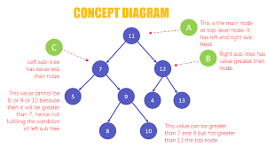
Key Properties
- Binary Structure: Each node has at most two children.
- Ordering: Left subtree < Node < Right subtree for all nodes.
- Unique Elements: Typically, all node values are distinct.
- Efficiency: Provides efficient insertion, deletion, and search operations.
- In-order Traversal: Produces sorted output.
Basic Components
- Node: Contains data and references to left and right children.
- Root: The topmost node of the tree.
- Leaf: A node with no children.
Basic Operations
- Insertion: Add a new node while maintaining BST properties.
- Deletion: Remove a node while maintaining BST properties.
- Search: Find a node with a specific value.
- Traversal: In-order, Pre-order, Post-order.
Time Complexity
- Average Case (balanced tree):
- Search: O(log n)
- Insertion: O(log n)
- Deletion: O(log n)
- Worst Case (unbalanced tree):
- Search: O(n)
- Insertion: O(n)
- Deletion: O(n)
Memory Usage
- Memory = (size of data + size of two pointers) * (number of nodes)
Advantages
- Efficient searching, insertion, and deletion (in balanced trees)
- Maintains sorted data structure
- Allows for in-order traversal to get sorted output
- Flexible size (can grow or shrink dynamically)
Disadvantages
- Performance degrades if tree becomes unbalanced
- No constant-time operations (unlike arrays)
- More complex to implement than simple linear data structures
Common Use Cases
- Implementing symbol tables in compilers
- Database indexing
- Implementing associative arrays
- Sorting algorithms (tree sort)
- Expression evaluation
Real-World Applications of Binary Search Trees
Binary Search Trees (BSTs) are versatile data structures that find applications in various domains due to their efficient searching, insertion, and deletion operations. Here are some real-world problems that can be solved or optimized using BSTs:
-
File System Organization
- Problem: Efficiently manage and search through directory structures.
- BST Solution: Represent the file system hierarchy, allowing for quick file/folder lookups.
-
Database Indexing
- Problem: Speed up database queries on specific fields.
- BST Solution: Create index structures (often B-trees, a variation of BST) for faster data retrieval.
-
Autocomplete and Spell Checkers
- Problem: Quickly suggest words as users type.
- BST Solution: Store dictionary words in a BST for efficient prefix-based searching.
-
IP Routing Tables
- Problem: Efficiently route network packets based on IP addresses.
- BST Solution: Organize routing information for quick lookups during packet forwarding.
-
Compiler Symbol Tables
- Problem: Manage variable and function names during compilation.
- BST Solution: Store and quickly retrieve symbol information for efficient compilation.
-
Game Development: Scene Graphs
- Problem: Organize and render game objects efficiently.
- BST Solution: Represent hierarchical relationships between game objects for optimized rendering and collision detection.
-
Appointment Scheduling Systems
- Problem: Manage and query time slots efficiently.
- BST Solution: Organize appointments by time, allowing for quick insertion, deletion, and overlap checking.
-
Air Traffic Control Systems
- Problem: Track and manage multiple aircraft efficiently.
- BST Solution: Organize aircraft by altitude or position for quick updates and collision avoidance checks.
-
Stock Market Trading Systems
- Problem: Quickly process and match buy/sell orders.
- BST Solution: Organize orders by price for efficient matching and execution.
-
Hierarchical Data Representation
- Problem: Represent and query organizational structures or taxonomies.
- BST Solution: Model hierarchical relationships with efficient searching and updating capabilities.
-
Morse Code Decoding
- Problem: Efficiently translate Morse code to text.
- BST Solution: Represent Morse code dictionary for quick character lookups.
-
Implementing Associative Arrays
- Problem: Create key-value pair data structures with efficient operations.
- BST Solution: Use keys to organize data for quick insertion, deletion, and retrieval of values.
-
Priority Queues in Operating Systems
- Problem: Manage process scheduling with different priorities.
- BST Solution: Organize processes by priority for efficient selection of next process to run.
-
Geographical Information Systems (GIS)
- Problem: Efficiently store and query spatial data.
- BST Solution: Organize geographical data points for range queries and nearest neighbor searches.
-
Huffman Coding in Data Compression
- Problem: Generate optimal prefix codes for data compression.
- BST Solution: Construct and traverse Huffman trees for encoding and decoding.
Remember that in many of these applications, variations of BSTs like AVL trees, Red-Black trees, or B-trees might be used to ensure balanced structures and optimal performance in large-scale systems.
Variations
- AVL Tree: Self-balancing BST
- Red-Black Tree: Self-balancing BST with color properties
- Splay Tree: Self-adjusting BST that moves recently accessed elements closer to the root
- Treap: Randomized BST
Memory Techniques for Retention
- Visualization: Imagine a family tree where younger generations are always to the left, older to the right.
- Analogy: Compare to a dictionary, where words to the left come before, and to the right come after the current word.
- Acronym: LESS (Left Elements Smaller Subtree)
- Mnemonic: "Left less, right more, search faster than before"
Code Example (Python)
class Node:
def __init__(self, key):
self.key = key
self.left = None
self.right = None
class BinarySearchTree:
def __init__(self):
self.root = None
def insert(self, key):
self.root = self._insert_recursive(self.root, key)
def _insert_recursive(self, root, key):
if root is None:
return Node(key)
if key < root.key:
root.left = self._insert_recursive(root.left, key)
else:
root.right = self._insert_recursive(root.right, key)
return root
def search(self, key):
return self._search_recursive(self.root, key)
def _search_recursive(self, root, key):
if root is None or root.key == key:
return root
if key < root.key:
return self._search_recursive(root.left, key)
return self._search_recursive(root.right, key)
def inorder_traversal(self):
result = []
self._inorder_recursive(self.root, result)
return result
def _inorder_recursive(self, root, result):
if root:
self._inorder_recursive(root.left, result)
result.append(root.key)
self._inorder_recursive(root.right, result)
def delete(self, key):
self.root = self._delete_recursive(self.root, key)
def _delete_recursive(self, root, key):
if root is None:
return root
if key < root.key:
root.left = self._delete_recursive(root.left, key)
elif key > root.key:
root.right = self._delete_recursive(root.right, key)
else:
if root.left is None:
return root.right
elif root.right is None:
return root.left
temp = self._min_value_node(root.right)
root.key = temp.key
root.right = self._delete_recursive(root.right, temp.key)
return root
def _min_value_node(self, node):
current = node
while current.left is not None:
current = current.left
return current
# Usage example
bst = BinarySearchTree()
bst.insert(50)
bst.insert(30)
bst.insert(70)
bst.insert(20)
bst.insert(40)
bst.insert(60)
bst.insert(80)
print("Inorder traversal:", bst.inorder_traversal())
print("Search 40:", "Found" if bst.search(40) else "Not Found")
bst.delete(40)
print("Inorder traversal after deleting 40:", bst.inorder_traversal())
Remember: Implement and experiment with Binary Search Trees in your preferred programming language to reinforce your understanding!
Binary Search Tree (BST) Operations: Insert, Delete, Search
A Binary Search Tree (BST) is a binary tree data structure with the following properties:
- The left subtree of a node contains only nodes with keys less than the node's key.
- The right subtree of a node contains only nodes with keys greater than the node's key.
- Both the left and right subtrees must also be binary search trees.
1. Insert Operation
The insert operation adds a new node with a given key to the BST while maintaining its properties.
Algorithm:
- If the tree is empty, create a new node and set it as the root.
- If the tree is not empty, compare the key to be inserted with the root's key:
- If the key is less than the root's key, recursively insert into the left subtree.
- If the key is greater than the root's key, recursively insert into the right subtree.
- If the key already exists, typically no action is taken (assuming duplicate keys are not allowed).
Time Complexity: O(h), where h is the height of the tree.
2. Delete Operation
The delete operation removes a node with a given key from the BST while maintaining its properties.
Algorithm:
- Search for the node to be deleted.
- If the node is found, there are three cases:
a. Node has no children (leaf node):
- Simply remove the node. b. Node has one child:
- Replace the node with its child. c. Node has two children:
- Find the inorder successor (smallest node in the right subtree).
- Replace the node's key with the inorder successor's key.
- Delete the inorder successor.
Time Complexity: O(h), where h is the height of the tree.
3. Search Operation
The search operation finds a node with a given key in the BST.
Algorithm:
- Start at the root.
- Compare the search key with the current node's key:
- If they match, return the current node.
- If the search key is less than the current node's key, recursively search the left subtree.
- If the search key is greater than the current node's key, recursively search the right subtree.
- If the end of the tree is reached without finding the key, return null or indicate that the key was not found.
Time Complexity: O(h), where h is the height of the tree.
Note: In a balanced BST, the height h is approximately log(n), where n is the number of nodes. However, in the worst case (a skewed tree), h can be n, leading to O(n) time complexity for all operations.
Tree Traversals: In-order, Pre-order, Post-order
Tree traversal is the process of visiting (checking and/or updating) each node in a tree data structure, exactly once. Unlike linear data structures (Array, Linked List, Queues, Stacks, etc.) which have only one logical way to traverse them, trees can be traversed in different ways.
1. In-order Traversal
In an in-order traversal, we visit the left subtree, then the root, and finally the right subtree.
Algorithm:
- Recursively traverse the left subtree.
- Visit the root.
- Recursively traverse the right subtree.
Pseudocode:
inorder(node)
if node is null, return
inorder(node.left)
visit(node)
inorder(node.right)
Use Case:
In-order traversal is commonly used with Binary Search Trees (BST) as it visits nodes in ascending order.
2. Pre-order Traversal
In a pre-order traversal, we visit the root first, then the left subtree, and finally the right subtree.
Algorithm:
- Visit the root.
- Recursively traverse the left subtree.
- Recursively traverse the right subtree.
Pseudocode:
preorder(node)
if node is null, return
visit(node)
preorder(node.left)
preorder(node.right)
Use Case:
Pre-order traversal is used to create a copy of the tree or to get prefix expression on an expression tree.
3. Post-order Traversal
In a post-order traversal, we visit the left subtree, then the right subtree, and finally the root.
Algorithm:
- Recursively traverse the left subtree.
- Recursively traverse the right subtree.
- Visit the root.
Pseudocode:
postorder(node)
if node is null, return
postorder(node.left)
postorder(node.right)
visit(node)
Use Case:
Post-order traversal is used when we want to delete the tree or to get the postfix expression of an expression tree.
Comparison and Time Complexity
Consider this binary tree:
1
/ \
2 3
/ \
4 5
Traversal results:
- In-order: 4 2 5 1 3
- Pre-order: 1 2 4 5 3
- Post-order: 4 5 2 3 1
Time Complexity: All three traversals have a time complexity of O(n), where n is the number of nodes in the tree, as they visit each node exactly once.
Space Complexity: O(h) for the recursive call stack, where h is the height of the tree. In the worst case of a skewed tree, this could be O(n).
Note: These traversals can also be implemented iteratively using a stack, which can be beneficial in certain scenarios, especially when dealing with very deep trees where recursive approaches might lead to stack overflow.
Graph Data Structure
Definition
A Graph is a non-linear data structure consisting of vertices (or nodes) and edges that connect these vertices. It is used to represent relationships between pairs of objects.
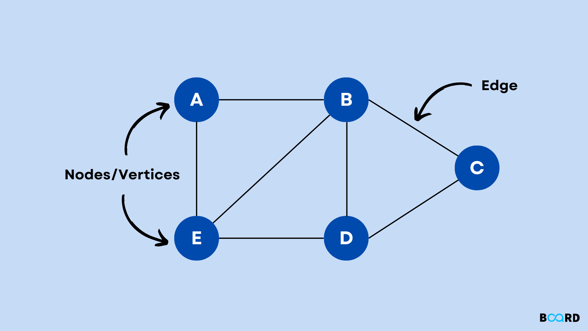
Key Properties
- Vertices: The fundamental units of the graph.
- Edges: Connections between pairs of vertices.
- Direction: Graphs can be directed (edges have direction) or undirected.
- Weight: Edges can have weights to represent costs, distances, etc.
- Connectivity: A graph can be connected or disconnected.
- Cyclicity: A graph can be cyclic or acyclic.
Types of Graphs
- Undirected Graph: Edges have no direction.
- Directed Graph (Digraph): Edges have direction.
- Weighted Graph: Edges have associated weights.
- Complete Graph: Every vertex is connected to every other vertex.
- Bipartite Graph: Vertices can be divided into two disjoint sets.
- Tree: A connected acyclic graph.
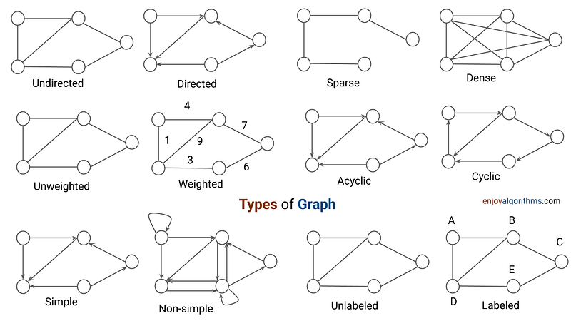
Basic Components
- Vertex: A node in the graph.
- Edge: A connection between two vertices.
- Path: A sequence of vertices connected by edges.
- Cycle: A path that starts and ends at the same vertex.
Basic Operations
- Add Vertex: Insert a new vertex into the graph.
- Add Edge: Add a new edge between two vertices.
- Remove Vertex: Delete a vertex and all its incident edges.
- Remove Edge: Delete an edge between two vertices.
- Graph Traversal: Visit all vertices in a graph (BFS, DFS).
- Search: Find a path between two vertices.
Representations
- Adjacency Matrix: 2D array where rows and columns represent vertices.
- Adjacency List: Array of lists, each representing connections of a vertex.
- Edge List: List of all edges in the graph.
Time Complexity (for V vertices and E edges)
- Adjacency Matrix:
- Add Vertex: O(V^2)
- Add Edge: O(1)
- Remove Vertex: O(V^2)
- Remove Edge: O(1)
- Query: O(1)
- Storage: O(V^2)
- Adjacency List:
- Add Vertex: O(1)
- Add Edge: O(1)
- Remove Vertex: O(V + E)
- Remove Edge: O(E)
- Query: O(V)
- Storage: O(V + E)
Advantages
- Model real-world relationships and networks
- Solve complex problems like shortest path, network flow
- Flexible structure for representing various types of data
- Efficient for certain operations depending on representation
Disadvantages
- Can be complex to implement and manage
- Some operations can be inefficient for large graphs
- Memory intensive, especially for dense graphs
Common Use Cases
- Social Networks (Facebook friends, LinkedIn connections)
- Geographic Maps and Navigation Systems
- Computer Networks and Communication Systems
- Recommendation Systems
- Dependency Resolution in Software Engineering
- Circuit Design in Electronics
Real-World Applications of Graph and Tree Data Structures
-
Social Networks
- Friend recommendations
- Influence analysis
- Community detection
- Shortest path between two users
-
Transportation and Navigation
- GPS and route planning
- Traffic flow optimization
- Airline flight paths
- Public transit systems
-
Computer Networks
- Internet routing protocols
- Network topology analysis
- Data packet routing
- Network flow optimization
-
Biology and Genetics
- Phylogenetic trees (evolutionary relationships)
- Protein interaction networks
- Gene regulatory networks
- Ecological food webs
-
Computer Science and Software Engineering
- File system hierarchies
- Syntax trees in compilers
- Dependency resolution in package managers
- State machines and game trees
-
Artificial Intelligence and Machine Learning
- Decision trees in machine learning
- Knowledge representation
- Neural networks
- Game-playing algorithms (e.g., chess, Go)
-
Business and Organization
- Company hierarchies
- Supply chain management
- Project management (PERT charts)
- Customer relationship mapping
-
Web Technologies
- Web crawling and indexing
- DOM (Document Object Model) in web browsers
- Website sitemaps
- Hyperlink structure analysis
-
Telecommunications
- Call routing in telephone networks
- Network capacity planning
- Cellular tower placement
These applications demonstrate the versatility and power of graph and tree data structures in modeling and solving complex real-world problems across various domains. The ability to represent relationships, hierarchies, and networks makes these structures fundamental tools in computer science and beyond.
Algorithms
- Breadth-First Search (BFS): Level-wise traversal
- Depth-First Search (DFS): Explore as far as possible along branches
- Dijkstra's Algorithm: Find shortest paths in weighted graphs
- Bellman-Ford Algorithm: Find shortest paths with negative weights
- Floyd-Warshall Algorithm: All pairs shortest paths
- Kruskal's and Prim's Algorithms: Minimum Spanning Tree
- Topological Sorting: Ordering of vertices in a directed acyclic graph
Memory Techniques for Retention
- Visualization: Imagine a social network diagram with people as nodes and friendships as edges.
- Analogy: Compare to a road map where cities are vertices and roads are edges.
- Acronym: VENOM (Vertices and Edges in a Network Object Model)
- Mnemonic: "Vertices vex, edges express, in graphs we connect and progress"
Code Example (Python)
from collections import defaultdict
class Graph:
def __init__(self):
self.graph = defaultdict(list)
def add_edge(self, u, v):
self.graph[u].append(v)
def bfs(self, start):
visited = set()
queue = [start]
visited.add(start)
while queue:
vertex = queue.pop(0)
print(vertex, end=" ")
for neighbor in self.graph[vertex]:
if neighbor not in visited:
visited.add(neighbor)
queue.append(neighbor)
def dfs_util(self, v, visited):
visited.add(v)
print(v, end=" ")
for neighbor in self.graph[v]:
if neighbor not in visited:
self.dfs_util(neighbor, visited)
def dfs(self, start):
visited = set()
self.dfs_util(start, visited)
# Usage example
g = Graph()
g.add_edge(0, 1)
g.add_edge(0, 2)
g.add_edge(1, 2)
g.add_edge(2, 0)
g.add_edge(2, 3)
g.add_edge(3, 3)
print("BFS starting from vertex 2:")
g.bfs(2)
print("\nDFS starting from vertex 2:")
g.dfs(2)
Hash Table (Hash Map) Data Structure
Definition
A Hash Table is a data structure that implements an associative array abstract data type, a structure that can map keys to values. It uses a hash function to compute an index into an array of buckets or slots, from which the desired value can be found.
Key Properties
- Key-Value Pairs: Stores data as key-value pairs.
- Hash Function: Uses a hash function to map keys to array indices.
- Collision Resolution: Handles situations where different keys hash to the same index.
- Dynamic Sizing: Can resize to maintain efficiency as the number of elements grows.
- Load Factor: Ratio of occupied slots to total slots, affects performance.
Basic Components
- Hash Function: Converts keys into array indices.
- Array: Stores the key-value pairs.
- Collision Resolution Method: Handles multiple keys mapping to the same index.
Basic Operations
- Insert: Add a new key-value pair.
- Delete: Remove a key-value pair.
- Search: Find the value associated with a given key.
- Update: Modify the value associated with a given key.
Time Complexity
- Average Case (with a good hash function):
- Insert: O(1)
- Delete: O(1)
- Search: O(1)
- Worst Case (many collisions):
- All operations: O(n)
Space Complexity
- O(n), where n is the number of key-value pairs stored
Collision Resolution Techniques
- Chaining: Each array index points to a linked list of entries.
- Open Addressing:
- Linear Probing: Check next slot sequentially.
- Quadratic Probing: Check slots at quadratic intervals.
- Double Hashing: Use a second hash function.
Advantages
- Fast average-case access, insertion, and deletion (O(1))
- Flexible keys (can use strings, objects, etc. as keys)
- Efficient for large datasets when properly tuned
- Implements dictionary/map abstract data type
Disadvantages
- Poor worst-case performance
- May require resizing, which is expensive
- Not efficient for small datasets
- No ordering of keys
Common Use Cases
- Database indexing
- Caches (e.g., web browser cache)
- Symbol tables in compilers
- Spell checkers
- Implementing associative arrays
- Counting distinct elements
Real-World Applications of Hash Maps
- Web Development and Databases
- Caching frequently accessed data to reduce database load
- Session storage in web applications
- URL shorteners
- Implementing database indexes for faster querying
- Network and Systems
- IP address to domain name mapping (DNS lookups)
- Load balancing in distributed systems
- Implementing routing tables in network routers
- Storing configuration settings for quick access
- Computer Science and Programming
- Symbol tables in compilers and interpreters
- Implementing sets and dictionaries in programming languages
- Memoization in dynamic programming to store computed results
- Counting sort algorithm implementation
- Data Processing and Analytics
- Counting word frequencies in large text documents
- Deduplication of data entries
- Implementing sparse matrices
- Histogram creation for data analysis
- Cybersecurity
- Password hashing and verification
- Bloom filters for malware detection
- Storing and checking against blacklists (e.g., IP addresses, email domains)
- Implementing hash-based message authentication codes (HMAC)
- Gaming
- Storing game states for quick save/load operations
- Implementing inventory systems in RPGs
- Collision detection in 2D games
- Caching pre-computed game scenarios
- File Systems and Operating Systems
- File system implementation (mapping file names to inodes)
- Implementing disk cache for faster file access
- Process and thread management in operating systems
- Storing environment variables
- E-commerce and Finance
- Shopping cart implementation in online stores
- Currency conversion tables
- Implementing stock symbol lookups
- Caching product information for quick display
- Social Media and Communication
- Storing user profiles for quick access
- Implementing friend lists or follower systems
- Message deduplication in chat applications
- Caching recent posts or tweets
- Artificial Intelligence and Machine Learning
- Feature hashing in machine learning models
- Implementing associative memories in neural networks
- Storing and retrieving trained model parameters
- Implementing efficient nearest neighbor search algorithms
- Graphics and Multimedia
- Color mapping in image processing
- Texture caching in 3D rendering engines
- Storing and retrieving media metadata
- Implementing sprite sheets in 2D game development
- Biotechnology and Bioinformatics
- DNA sequence analysis (k-mer counting)
- Protein structure prediction (storing intermediate results)
- Implementing genome databases for quick lookups
- Drug discovery (molecular fingerprinting)
Variations
- Bloom Filter: Space-efficient probabilistic data structure
- Cuckoo Hashing: Uses multiple hash functions for better worst-case performance
- Perfect Hashing: Achieves O(1) worst-case lookup time for static sets
Memory Techniques for Retention
- Visualization: Imagine a library where books (values) are placed on shelves (array slots) based on a code (hash) derived from their titles (keys).
- Analogy: Compare to a valet parking system where car placement is determined by a function of the license plate number.
- Acronym: HASH (Hashed Array Stores Haplessly)
- Mnemonic: "Key to index, value in place, constant time access, at lightning pace"
Code Example (Python)
class HashTable:
def __init__(self, size=10):
self.size = size
self.table = [[] for _ in range(self.size)]
def _hash(self, key):
return hash(key) % self.size
def insert(self, key, value):
index = self._hash(key)
for item in self.table[index]:
if item[0] == key:
item[1] = value
return
self.table[index].append([key, value])
def get(self, key):
index = self._hash(key)
for item in self.table[index]:
if item[0] == key:
return item[1]
raise KeyError(key)
def remove(self, key):
index = self._hash(key)
for i, item in enumerate(self.table[index]):
if item[0] == key:
del self.table[index][i]
return
raise KeyError(key)
def __str__(self):
return str(self.table)
# Usage example
ht = HashTable()
ht.insert("apple", 5)
ht.insert("banana", 7)
ht.insert("orange", 3)
print(ht.get("banana")) # Output: 7
ht.remove("apple")
print(ht) # Output: [[], [['banana', 7]], [], [], [], [], [], [], [], [['orange', 3]]]
Unit 4 - Searching & Sorting Algorithms
The Importance of Algorithms in Computer Science
Algorithms are the backbone of computer science and play a crucial role in solving complex problems efficiently. They are step-by-step procedures designed to perform a specific task or solve a particular problem. Among the vast array of algorithmic concepts, searching and sorting stand out as fundamental operations that are ubiquitous in computer science and real-world applications.
Why Algorithms Matter
-
Efficiency: Algorithms provide systematic ways to solve problems, often reducing the time and resources required to complete tasks. A well-designed algorithm can make the difference between a program that runs in seconds and one that takes hours or even days.
-
Scalability: As data sets grow larger, the importance of efficient algorithms becomes more pronounced. An algorithm that works well for small amounts of data may become impractical for large-scale applications. Understanding algorithms helps in creating solutions that scale well.
-
Problem-Solving Skills: Learning about algorithms enhances logical thinking and problem-solving abilities. It teaches students how to break down complex problems into manageable steps.
-
Optimization: Algorithms help in optimizing processes, whether in software development, data analysis, or system design. This leads to better performance, reduced costs, and improved user experiences.
Importance of Searching Algorithms
-
Data Retrieval: In an era of big data, the ability to quickly find specific information is crucial. Search algorithms are used in databases, file systems, and information retrieval systems.
-
Decision Making: Many applications require fast decision-making based on finding specific data points. For example, in a navigation system, quickly finding the shortest path is essential.
-
Pattern Matching: Searching algorithms are fundamental in pattern matching, which is used in areas like DNA sequence analysis, text processing, and computer vision.
-
Optimization Problems: Many optimization problems involve searching through a space of possible solutions to find the best one.
Importance of Sorting Algorithms
-
Data Organization: Sorted data is easier to search through, analyze, and understand. It's a prerequisite for many other algorithms and data structures.
-
Efficiency in Other Algorithms: Many algorithms, including searching algorithms, become more efficient when operating on sorted data.
-
Data Analysis and Visualization: Sorted data is essential for various statistical operations and data visualization techniques.
-
Database Operations: Sorting is crucial in database management systems for indexing, query optimization, and data retrieval.
Why You Need to Learn Searching and Sorting
-
Fundamental Building Blocks: Understanding these basic algorithms provides a foundation for learning more complex algorithmic concepts.
-
Performance Analysis: Studying different searching and sorting algorithms helps students understand algorithm analysis, including concepts like time and space complexity.
-
Problem-Solving Techniques: These algorithms introduce important problem-solving techniques like divide-and-conquer, recursion, and iterative improvement.
-
Real-World Applications: Knowledge of searching and sorting is directly applicable in many real-world scenarios and is often tested in technical interviews.
-
Algorithm Design Skills: Learning these algorithms helps develop skills in designing and improving algorithms for other problems.
-
Understanding Trade-offs: Different searching and sorting algorithms have various strengths and weaknesses. Understanding these trade-offs is crucial for choosing the right algorithm for a given situation.
Linear Search Algorithm
1. Concept
Linear search, also known as sequential search, is one of the simplest searching algorithms. It works by sequentially checking each element in a collection until a match is found or the entire collection has been searched.
2. How Linear Search Works
The algorithm follows these steps:
- Start from the first element of the array.
- Compare the current element with the target value.
- If the current element matches the target, return its index.
- If not, move to the next element.
- Repeat steps 2-4 until the element is found or the end of the array is reached.
- If the element is not found, return a signal (often -1) or False to indicate the element is not in the array.
HOMEWORK:
- Draw a flowchart for Linear Search algorithm
- Write Psuedocode for Linear Search algorithm
3. Time and Space Complexity
Time Complexity
- Best Case: O(1) - when the target element is at the beginning of the array
- Worst Case: O(n) - when the target element is at the end or not in the array
- Average Case: O(n) - on average, we might need to search half the array
Space Complexity
- O(1) - linear search uses a constant amount of extra space regardless of input size
4. When to Use & When Not to Use Linear Search
Use Linear Search When:
- The array is small
- The array is unsorted
- You need to search for an element only once
- Simplicity is more important than speed
- Hardware constraints favor simple algorithms
Avoid Linear Search When:
- The array is large and sorted (use binary search instead)
- You need to perform multiple searches on the same array (consider sorting first)
- Performance is critical and the dataset is large
5. Implementing Linear Search in Python
One of the implementation in Python:
def linear_search(arr, target):
for i in range(len(arr)):
if arr[i] == target:
return i # Return the index if the element is found
return -1 # Return -1 if the element is not found
# Example usage
my_array = [5, 2, 9, 1, 7, 6, 3]
result = linear_search(my_array, 7)
print(f"Element found at index: {result}")
6. Example Problem and Solution
Problem Statement
A teacher has a list of student IDs and needs to find if a particular student is present in the class. Write a function that takes a list of student IDs and a target ID, and returns whether the student is present and their position in the list (1-indexed).
Solution
def find_student(student_ids, target_id):
for i, student_id in enumerate(student_ids, start=1):
if student_id == target_id:
return f"Student with ID {target_id} is present at position {i}."
return f"Student with ID {target_id} is not present in the class."
# Example usage
class_ids = [1001, 1002, 1003, 1004, 1005, 1006, 1007]
target_student = 1005
result = find_student(class_ids, target_student)
print(result)
# Test with a student not in the class
missing_student = 1010
result = find_student(class_ids, missing_student)
print(result)
This implementation uses linear search to find the student ID in the list. It returns the position (1-indexed for easier understanding by non-programmers) if the student is found, or a message indicating the student is not present.
The time complexity remains O(n) in the worst case, where n is the number of students in the class. This approach is suitable for small to medium-sized classes where the simplicity of implementation outweighs the need for optimized search performance.
Binary Search
1. Concept
Binary search is a highly efficient searching algorithm used to find a specific element within a sorted array. It works on the principle of divide and conquer, repeatedly dividing the search interval in half until the desired element is found or it's determined that the element doesn't exist in the array.
2. How Binary Search Works
- Start with a sorted array.
- Define two pointers:
left(starting at the first element) andright(starting at the last element). - Calculate the middle index:
mid = (left + right) // 2. - Compare the middle element with the target value:
- If equal, the search is successful.
- If the target is less than the middle element, search the left half (set
right = mid - 1). - If the target is greater than the middle element, search the right half (set
left = mid + 1).
- Repeat steps 3-4 until the element is found or the search space is exhausted (
left > right).
3. Time and Space Complexity
- Time Complexity:
- Best case: O(1) - when the middle element is the target
- Average case: O(log n)
- Worst case: O(log n)
- Space Complexity: O(1) - constant space is used
The logarithmic time complexity makes binary search significantly faster than linear search for large datasets.
4. When to Use & When Not to Use Binary Search
Use Binary Search when:
- The array is sorted
- The array is large, and efficiency is crucial
Don't Use Binary Search when:
- The array is unsorted (sorting first may be costlier than a linear search)
- The array is small (linear search might be faster due to simplicity)
- The array is frequently modified (maintaining sorted order can be expensive)
- You need to find all occurrences of an element (binary search finds only one)
5. Implementing Binary Search in Python
Implementation in Python:
def binary_search(arr, target):
left, right = 0, len(arr) - 1
while left <= right:
mid = (left + right) // 2
if arr[mid] == target:
return mid # Target found, return its index
elif arr[mid] < target:
left = mid + 1 # Target is in the right half
else:
right = mid - 1 # Target is in the left half
return -1 # Target not found
6. Example Scenario: Finding a Student's Score
Problem Statement
Problem: A school maintains a sorted list of student scores. Given a student's score, find their rank in the class (assuming no two students have the same score).
Solution
def find_rank(scores, target_score):
left, right = 0, len(scores) - 1
while left <= right:
mid = (left + right) // 2
if scores[mid] == target_score:
return len(scores) - mid # Rank is position from the end
elif scores[mid] < target_score:
right = mid - 1 # Look in the left half (higher scores)
else:
left = mid + 1 # Look in the right half (lower scores)
# If the exact score isn't found, return the rank it would have
return len(scores) - right
# Example usage
scores = [95, 90, 85, 80, 75, 70, 65, 60] # Sorted in descending order
student_score = 82
rank = find_rank(scores, student_score)
print(f"A student with a score of {student_score} would rank {rank} in the class.")
In this example, we use binary search to efficiently find where a given score would fit in the sorted list of scores. The rank is determined by the position from the end of the list, as higher scores typically indicate better ranks.
This implementation showcases how binary search can be adapted to solve real-world problems efficiently, especially when dealing with sorted data.
Depth-First Search
Concept
Depth-First Search (DFS) is a fundamental graph traversal algorithm used in computer science and artificial intelligence. It explores a graph or tree data structure by going as deep as possible along each branch before backtracking. This approach allows DFS to reach the leaf nodes of a graph quickly, making it useful for many applications such as pathfinding, topological sorting, and cycle detection.
The key characteristic of DFS is its "depth-first" nature: it prioritizes exploring as far as possible along each branch before exploring other branches. This behavior is analogous to exploring a maze by following each path to its end before backtracking and trying a different path.
How DFS Works - Recursive & Iterative
Recursive DFS
The recursive implementation of DFS is elegant and intuitive, mirroring the algorithm's natural depth-first behavior:
- Start at a chosen node (often called the root in tree structures).
- Mark the current node as visited.
- For each unvisited neighbor of the current node: a. Recursively apply DFS to that neighbor.
- If all neighbors are visited, the function returns (effectively backtracking).
This process naturally creates a depth-first traversal as the recursion pushes deeper into the graph before unwinding.
Iterative DFS
The iterative version uses a stack to simulate the recursive call stack:
- Start at the chosen node and push it onto a stack.
- While the stack is not empty: a. Pop a node from the stack and mark it as visited. b. Push all unvisited neighbors of this node onto the stack.
- Repeat step 2 until the stack is empty.
The stack ensures that we explore deeper paths before wider ones, maintaining the depth-first property.
Time / Space Complexity - Recursive and Iterative
Time Complexity
Both recursive and iterative implementations have the same time complexity:
- O(V + E) for an adjacency list representation
- O(V^2) for an adjacency matrix representation
Where V is the number of vertices and E is the number of edges in the graph.
This is because each vertex and edge will be explored once.
Space Complexity
Recursive DFS
- Worst case: O(V) where V is the number of vertices
- This occurs in the case of a skewed graph (like a linked list)
- The space is used by the call stack
Iterative DFS
- Worst case: O(V) where V is the number of vertices
- This space is used by the explicit stack data structure
In practice, the iterative version often has better space efficiency, especially for very deep graphs, as it avoids potential stack overflow issues.
When to Use & When Not to Use DFS - Recursive and Iterative
When to Use DFS
- Pathfinding in maze-like problems
- Topological sorting
- Detecting cycles in graphs
- Solving puzzles with only one solution (e.g., sudoku)
- Generating permutations or combinations
Recursive DFS is preferred when:
- The graph is known to be shallow
- The solution is known to be far from the root
- The problem naturally fits a recursive formulation
- Simplicity of implementation is prioritized
Iterative DFS is preferred when:
- The graph might be very deep
- Memory usage is a concern (to avoid stack overflow)
- You need more control over the traversal process
When Not to Use DFS
- Finding the shortest path (BFS is usually better)
- When you need to search level by level
- When the graph is very deep and recursive DFS might cause stack overflow
- When you need to find all solutions, not just one (BFS might be more suitable)
Implementing DFS in Python - Recursive and Iterative
Recursive DFS Implementation
def dfs_recursive(graph, node, visited=None):
if visited is None:
visited = set()
visited.add(node)
print(node, end=' ') # Process the node
for neighbor in graph[node]:
if neighbor not in visited:
dfs_recursive(graph, neighbor, visited)
# Example usage
graph = {
'A': ['B', 'C'],
'B': ['D', 'E'],
'C': ['F'],
'D': [],
'E': ['F'],
'F': []
}
print("Recursive DFS:")
dfs_recursive(graph, 'A')
Iterative DFS Implementation
def dfs_iterative(graph, start):
visited = set()
stack = [start]
while stack:
node = stack.pop()
if node not in visited:
visited.add(node)
print(node, end=' ') # Process the node
# Add neighbors to stack in reverse order
# to match recursive DFS output
stack.extend(reversed(graph[node]))
# Example usage
print("\nIterative DFS:")
dfs_iterative(graph, 'A')
Scenario Problem: Solving a Maze using DFS
Let's solve a maze problem using iterative DFS. The maze will be represented as a 2D grid where:
- 0 represents a free cell
- 1 represents a wall
- 2 represents the starting point
- 3 represents the exit
Our task is to find a path from the start to the exit.
def solve_maze(maze):
def is_valid(x, y):
return 0 <= x < len(maze) and 0 <= y < len(maze[0]) and maze[x][y] != 1
def get_neighbors(x, y):
return [(x+1, y), (x-1, y), (x, y+1), (x, y-1)]
start = None
for i in range(len(maze)):
for j in range(len(maze[0])):
if maze[i][j] == 2:
start = (i, j)
break
if start:
break
stack = [start]
visited = set()
parent = {}
while stack:
x, y = stack.pop()
if maze[x][y] == 3: # Exit found
path = []
while (x, y) != start:
path.append((x, y))
x, y = parent[(x, y)]
path.append(start)
return path[::-1]
if (x, y) not in visited:
visited.add((x, y))
for nx, ny in get_neighbors(x, y):
if is_valid(nx, ny) and (nx, ny) not in visited:
stack.append((nx, ny))
parent[(nx, ny)] = (x, y)
return None # No path found
# Example maze
maze = [
[0, 0, 0, 0, 0],
[1, 1, 0, 1, 0],
[0, 0, 0, 0, 0],
[0, 1, 1, 1, 0],
[0, 0, 0, 1, 3],
[2, 1, 0, 0, 0]
]
path = solve_maze(maze)
if path:
print("Path found:", path)
else:
print("No path found")
# Visualize the path
def print_maze_with_path(maze, path):
for i in range(len(maze)):
for j in range(len(maze[0])):
if (i, j) in path:
print("*", end=" ")
else:
print(maze[i][j], end=" ")
print()
print("\nMaze with path:")
print_maze_with_path(maze, path)
This implementation uses iterative DFS to solve the maze. It starts from the starting point (2), explores possible paths using a stack, and backtracks when it hits a wall or a visited cell. When it reaches the exit (3), it reconstructs and returns the path. The visualization shows the path with asterisks (*).
This example demonstrates how DFS can be applied to solve real-world problems like navigating through a maze, showcasing its strength in pathfinding applications.
BreadthFirst Search
Concept
Breadth-First Search (BFS) is a fundamental graph traversal algorithm used in computer science and artificial intelligence. Unlike Depth-First Search (DFS), which explores as far as possible along each branch before backtracking, BFS explores all the neighbor nodes at the present depth prior to moving on to the nodes at the next depth level.
The key characteristic of BFS is its "breadth-first" nature: it visits all the vertices at the same level before moving to the vertices at the next level. This behavior is analogous to how a ripple spreads out in a pond, reaching all points at a certain distance before moving further.
How BFS Works - Iterative
BFS is typically implemented iteratively using a queue data structure. Here's how it works:
- Start at a chosen node (often called the root in tree structures).
- Mark the current node as visited and enqueue it.
- While the queue is not empty:
a. Dequeue a node from the front of the queue.
b. Explore all unvisited neighbors of this node:
- Mark each neighbor as visited.
- Enqueue each neighbor.
- Repeat step 3 until the queue is empty.
This process ensures that we explore all nodes at a given depth before moving to the next depth level.
Note: While it's possible to implement BFS recursively, it's not common or practical due to the nature of the algorithm. The iterative implementation using a queue is the standard approach.
Time / Space Complexity
Time Complexity
- O(V + E) for an adjacency list representation
- O(V^2) for an adjacency matrix representation
Where V is the number of vertices and E is the number of edges in the graph.
This is because each vertex and edge will be explored once.
Space Complexity
- O(V) where V is the number of vertices
The space is used by the queue data structure. In the worst case, the queue might need to store all vertices of the graph.
When to Use & When Not to Use BFS
When to Use BFS
- Finding the shortest path in an unweighted graph
- Level-order traversal of a tree
- Finding all nodes within one connected component
- Testing if a graph is bipartite
- Finding the shortest path between two nodes
- Web crawling
- Social networking features (e.g., finding all friends within a certain degree of connection)
When Not to Use BFS
- When memory is a constraint (as it may need to store many nodes)
- When exploring deeper paths in a graph is prioritized
- When the solution is likely to be far from the root (DFS might be faster)
- When working with infinite graphs or trees (as BFS expands in all directions)
Implementing BFS in Python
Here's a Python implementation of BFS:
from collections import deque
def bfs(graph, start):
visited = set()
queue = deque([start])
visited.add(start)
while queue:
vertex = queue.popleft()
print(vertex, end=' ') # Process the node
for neighbor in graph[vertex]:
if neighbor not in visited:
visited.add(neighbor)
queue.append(neighbor)
# Example usage
graph = {
'A': ['B', 'C'],
'B': ['D', 'E'],
'C': ['F'],
'D': [],
'E': ['F'],
'F': []
}
print("BFS traversal:")
bfs(graph, 'A')
Example Problem: Shortest Path in a Maze
Let's solve a maze problem using BFS to find the shortest path. The maze will be represented as a 2D grid where:
- 0 represents a free cell
- 1 represents a wall
- 2 represents the starting point
- 3 represents the exit
Our task is to find the shortest path from the start to the exit.
from collections import deque
def solve_maze_bfs(maze):
def is_valid(x, y):
return 0 <= x < len(maze) and 0 <= y < len(maze[0]) and maze[x][y] != 1
def get_neighbors(x, y):
return [(x+1, y), (x-1, y), (x, y+1), (x, y-1)]
start = None
for i in range(len(maze)):
for j in range(len(maze[0])):
if maze[i][j] == 2:
start = (i, j)
break
if start:
break
queue = deque([start])
visited = set([start])
parent = {}
while queue:
x, y = queue.popleft()
if maze[x][y] == 3: # Exit found
path = []
while (x, y) != start:
path.append((x, y))
x, y = parent[(x, y)]
path.append(start)
return path[::-1]
for nx, ny in get_neighbors(x, y):
if is_valid(nx, ny) and (nx, ny) not in visited:
visited.add((nx, ny))
queue.append((nx, ny))
parent[(nx, ny)] = (x, y)
return None # No path found
# Example maze
maze = [
[0, 0, 0, 0, 0],
[1, 1, 0, 1, 0],
[0, 0, 0, 0, 0],
[0, 1, 1, 1, 0],
[0, 0, 0, 1, 3],
[2, 1, 0, 0, 0]
]
path = solve_maze_bfs(maze)
if path:
print("Shortest path found:", path)
print("Path length:", len(path) - 1) # -1 because we don't count the starting position
else:
print("No path found")
# Visualize the path
def print_maze_with_path(maze, path):
for i in range(len(maze)):
for j in range(len(maze[0])):
if (i, j) in path:
print("*", end=" ")
else:
print(maze[i][j], end=" ")
print()
print("\nMaze with shortest path:")
print_maze_with_path(maze, path)
This implementation uses BFS to solve the maze. It starts from the starting point (2), explores possible paths using a queue, and keeps track of the parent of each cell. When it reaches the exit (3), it reconstructs and returns the shortest path. The visualization shows the path with asterisks (*).
This example demonstrates how BFS can be applied to find the shortest path in a maze, showcasing its strength in finding optimal solutions in unweighted graphs.
Bubble Sort
1. Concept
Bubble sort is a simple sorting algorithm that repeatedly steps through a list, compares adjacent elements, and swaps them if they are in the wrong order. The algorithm gets its name from the way smaller elements "bubble" to the top of the list with each iteration.
2. How Does Bubble Sort Work
Bubble sort works by repeatedly traversing the list from left to right, comparing adjacent elements, and swapping them if they are in the wrong order. This process is repeated for each element in the list until no more swaps are needed, which indicates that the list is sorted.
The steps are as follows:
- Start with the first element (index 0).
- Compare the current element with the next element.
- If the current element is greater than the next element, swap them.
- Move to the next element and repeat steps 2-3 until the end of the list.
- Repeat steps 1-4 for each element in the list.
- The algorithm stops when no more swaps are performed in a full pass.
3. Time / Space Complexity
Time Complexity:
- Worst-case: O(n²) - when the array is in reverse order
- Average-case: O(n²)
- Best-case: O(n) - when the array is already sorted
Space Complexity:
- O(1) - Bubble sort is an in-place sorting algorithm, meaning it doesn't require any extra space proportional to the input size.
4. When to Use & When Not to Use Bubble Sort
When to use:
- For small datasets or nearly sorted lists
- When simplicity is preferred over efficiency
- In educational settings to teach basic sorting concepts
- When memory usage is a concern (due to its in-place nature)
When not to use:
- For large datasets (inefficient for big lists)
- In performance-critical applications
- When faster algorithms like QuickSort or MergeSort are available
- In production environments where efficiency is crucial
5. Implementing Bubble Sort in Python
Here's a Python implementation of the bubble sort algorithm:
def bubble_sort(arr):
n = len(arr)
for i in range(n):
# Flag to optimize the algorithm
swapped = False
# Last i elements are already in place
for j in range(0, n-i-1):
# Traverse the array from 0 to n-i-1
# Swap if the element found is greater than the next element
if arr[j] > arr[j+1]:
arr[j], arr[j+1] = arr[j+1], arr[j]
swapped = True
# If no swapping occurred, array is already sorted
if not swapped:
break
return arr
6. Scenario Problem and Solution
Problem: A teacher has a list of student scores and wants to sort them in ascending order to determine the class ranking.
Example:
def bubble_sort(scores):
n = len(scores)
for i in range(n):
swapped = False
for j in range(0, n-i-1):
if scores[j] > scores[j+1]:
scores[j], scores[j+1] = scores[j+1], scores[j]
swapped = True
if not swapped:
break
return scores
# List of student scores
student_scores = [78, 65, 90, 82, 70, 88, 85]
print("Original scores:", student_scores)
sorted_scores = bubble_sort(student_scores)
print("Sorted scores:", sorted_scores)
# Determine rankings
rankings = {score: rank for rank, score in enumerate(sorted(set(sorted_scores), reverse=True), 1)}
student_rankings = [rankings[score] for score in student_scores]
print("Student rankings:", student_rankings)
Output:
Original scores: [78, 65, 90, 82, 70, 88, 85]
Sorted scores: [65, 70, 78, 82, 85, 88, 90]
Student rankings: [5, 7, 1, 4, 6, 2, 3]
Insertion Sort
1. Concept
Insertion sort is a simple sorting algorithm that builds the final sorted array one item at a time. It's much like sorting a hand of playing cards. You start with one card and then insert each subsequent card into its proper position among the cards you've already sorted.
2. How Does Insertion Sort Work
Insertion sort works by virtually splitting the array into a sorted and an unsorted part. Values from the unsorted part are picked and placed in the correct position in the sorted part.
The steps are as follows:
- Start with the second element (index 1) as the key.
- Compare the key with the elements before it.
- If the element before the key is greater, move it one position ahead.
- Repeat step 3 until a smaller (or equal) element is found or the start of the array is reached.
- Place the key in the correct position.
- Repeat steps 1-5 for all elements in the array.
3. Time / Space Complexity
Time Complexity:
- Worst-case: O(n²) - when the array is in reverse order
- Average-case: O(n²)
- Best-case: O(n) - when the array is already sorted
Space Complexity:
- O(1) - Insertion sort is an in-place sorting algorithm, so it uses only a constant amount of extra space.
4. When to Use & When Not to Use Insertion Sort
When to use:
- For small datasets or nearly sorted lists
- When dealing with continuous inflow of numbers and they need to be kept sorted
- When memory usage is a concern (due to its in-place nature)
- For simplicity in implementation
When not to use:
- For large datasets (inefficient for big lists)
- In performance-critical applications with large amounts of data
- When faster algorithms like QuickSort or MergeSort are more suitable
- In scenarios where the data is completely unsorted and large
5. Implementing Insertion Sort in Python
Here's a Python implementation of the insertion sort algorithm:
def insertion_sort(arr):
for i in range(1, len(arr)):
key = arr[i]
j = i - 1
# Move elements of arr[0..i-1], that are greater than key,
# to one position ahead of their current position
while j >= 0 and key < arr[j]:
arr[j + 1] = arr[j]
j -= 1
arr[j + 1] = key
return arr
6. Example Problem
Problem: A librarian needs to sort a list of books by their publication year to arrange them chronologically on a shelf.
Example:
def insertion_sort(books):
for i in range(1, len(books)):
key = books[i]
j = i - 1
while j >= 0 and key['year'] < books[j]['year']:
books[j + 1] = books[j]
j -= 1
books[j + 1] = key
return books
# List of books with their titles and publication years
books = [
{"title": "To Kill a Mockingbird", "year": 1960},
{"title": "Pride and Prejudice", "year": 1813},
{"title": "1984", "year": 1949},
{"title": "The Great Gatsby", "year": 1925},
{"title": "The Catcher in the Rye", "year": 1951}
]
print("Original order:")
for book in books:
print(f"{book['title']} ({book['year']})")
sorted_books = insertion_sort(books)
print("\nSorted by year:")
for book in sorted_books:
print(f"{book['title']} ({book['year']})")
Output:
Original order:
To Kill a Mockingbird (1960)
Pride and Prejudice (1813)
1984 (1949)
The Great Gatsby (1925)
The Catcher in the Rye (1951)
Sorted by year:
Pride and Prejudice (1813)
The Great Gatsby (1925)
1984 (1949)
The Catcher in the Rye (1951)
To Kill a Mockingbird (1960)
This example demonstrates how insertion sort can be used to sort a list of books by their publication year, allowing the librarian to arrange them chronologically.
Quick Sort
1. Concept
Quicksort is a highly efficient, divide-and-conquer sorting algorithm. It works by selecting a 'pivot' element from the array and partitioning the other elements into two sub-arrays, according to whether they are less than or greater than the pivot. The sub-arrays are then sorted recursively.
2. How Does Quicksort Work
Quicksort follows these steps:
- Choose a pivot element from the array.
- Partition the array:
- Move all elements smaller than the pivot to its left.
- Move all elements larger than the pivot to its right.
- Recursively apply steps 1-2 to the sub-array of elements with smaller values and the sub-array of elements with larger values.
The base case of the recursion is arrays of size zero or one, which are always sorted.
3. Time / Space Complexity
Time Complexity:
- Worst-case: O(n²) - when the pivot is always the smallest or largest element
- Average-case: O(n log n)
- Best-case: O(n log n)
Space Complexity:
- Worst-case: O(n) - due to the recursive call stack
- Average-case: O(log n)
Note: The space complexity can be reduced to O(log n) by using tail recursion optimization.
4. When to Use & When Not to Use Quicksort
When to use:
- For large datasets where efficiency is crucial
- When average-case performance is more important than worst-case performance
- In situations where in-place sorting is beneficial to save memory
- When a good pivot selection strategy can be implemented
When not to use:
- When stability is required (preserving the relative order of equal elements)
- In systems where worst-case performance is critical
- For small datasets where simpler algorithms like insertion sort might be faster
- In memory-constrained environments where the recursive nature might be problematic
5. Implementing Quicksort in Python
Here's a Python implementation of the quicksort algorithm:
def quicksort(arr):
if len(arr) <= 1:
return arr
else:
pivot = arr[len(arr) // 2]
left = [x for x in arr if x < pivot]
middle = [x for x in arr if x == pivot]
right = [x for x in arr if x > pivot]
return quicksort(left) + middle + quicksort(right)
Note: This implementation is not in-place and uses extra space. An in-place version would be more memory-efficient but slightly more complex.
6. Scenario Problem and Solution
Problem: A teacher wants to rank students based on their total scores, which are calculated from multiple subjects. The scores need to be sorted in descending order to assign ranks.
Example:
def quicksort(arr):
if len(arr) <= 1:
return arr
else:
pivot = arr[len(arr) // 2]
left = [x for x in arr if x['total_score'] > pivot['total_score']]
middle = [x for x in arr if x['total_score'] == pivot['total_score']]
right = [x for x in arr if x['total_score'] < pivot['total_score']]
return quicksort(left) + middle + quicksort(right)
# List of students with their names and total scores
students = [
{"name": "Alice", "total_score": 385},
{"name": "Bob", "total_score": 350},
{"name": "Charlie", "total_score": 400},
{"name": "David", "total_score": 395},
{"name": "Eve", "total_score": 355}
]
print("Original order:")
for student in students:
print(f"{student['name']}: {student['total_score']}")
sorted_students = quicksort(students)
print("\nRanked order:")
for rank, student in enumerate(sorted_students, 1):
print(f"Rank {rank}: {student['name']} - {student['total_score']}")
Output:
Original order:
Alice: 385
Bob: 350
Charlie: 400
David: 395
Eve: 355
Ranked order:
Rank 1: Charlie - 400
Rank 2: David - 395
Rank 3: Alice - 385
Rank 4: Eve - 355
Rank 5: Bob - 350
This example demonstrates how quicksort can be used to efficiently rank students based on their total scores, sorting them in descending order.
Space Time Complexity - Asymptotic Notation
YouTube Video Explaining Big O
Introduction
In the world of computer science, particularly in the study of Data Structures and Algorithms, you'll often hear about "Big O notation."
1. Concept of Time & Space
1.1 Time Complexity
Time complexity is a way to describe how long an algorithm takes to run as the input size increases. It's not about measuring the actual time in seconds, but rather about counting the number of operations the algorithm performs.
Think of it like this: Imagine you're baking cookies. The time complexity would be like counting how many steps (mixing ingredients, shaping cookies, etc.) you need to perform to bake a certain number of cookies. As you bake more cookies, you might need more steps.
How to express the Time Complexity of an Algorithm:
We use Big O notation to express time complexity. It describes the worst-case scenario or the maximum number of operations an algorithm might need to perform.
Here are some common time complexities, from fastest to slowest:
- O(1) - Constant time
- O(log n) - Logarithmic time
- O(n) - Linear time
- O(n log n) - Linearithmic time
- O(n^2) - Quadratic time
- O(2^n) - Exponential time
- O(n!) - Factorial time
1.2 Space Complexity
Space complexity is about how much additional memory an algorithm needs to run as the input size increases. It's not about the space taken by the input itself, but the extra space the algorithm uses.
Think of it like this: When you're baking cookies, space complexity would be like measuring how many extra bowls, spoons, and baking sheets you need as you make more cookies.
The representation of Space Complexities is the same as that of Time Complexity - using Big O notaiton.
Here are some common time complexities, from fastest to slowest:
- O(1) - Constant space
- O(log n) - Logarithmic space
- O(n) - Linear space
- O(n log n) - Linearithmic space
- O(n^2) - Quadratic space
- O(2^n) - Exponential space
- O(n!) - Factorial space
2. Why Big O Notation?
Big O notation is a fundamental concept in computer science for several reasons:
-
Efficiency Analysis: It helps us analyze the efficiency of algorithms, allowing us to compare different approaches to solving a problem.
-
Scalability: It gives us insight into how an algorithm will perform as the input size grows, which is crucial for building systems that can handle large amounts of data.
-
Optimization: Understanding Big O helps developers optimize their code by choosing the most efficient algorithms for their specific use cases.
-
Standardized Communication: It provides a standardized way to discuss algorithm performance across the computer science community.
3. Best Case, Average Case, and Worst Case
When analyzing algorithms, we often consider three scenarios:
-
Best Case: The most favorable input scenario, resulting in the fastest possible execution time.
-
Average Case: The expected performance for a typical input.
-
Worst Case: The least favorable input scenario, resulting in the slowest execution time.
Big O notation typically describes the worst-case scenario, as it gives us an upper bound on the algorithm's performance. This ensures we're prepared for the most challenging situations our algorithm might face.
4. Mathematical Origins (Brief Overview)
Big O notation originated from mathematics, specifically from the field of asymptotic analysis. It was introduced by the German mathematician Paul Bachmann in 1894 and later popularized in computer science.
The "O" in Big O stands for "Order of," referring to the order of magnitude of the algorithm's performance. It describes how the runtime of an algorithm grows relative to the input size as the input size approaches infinity.
While the mathematical foundations are complex, in computer science, we use a simplified version that focuses on the dominant term of the function describing the algorithm's performance.
5 Examples - Time & Space Complexity
5.1 O(1) Time, O(1) Space - Constant Time and Space
def get_first_element(arr):
return arr[0] if arr else None
# Usage
result = get_first_element([1, 2, 3, 4, 5])
This function always performs one operation (accessing the first element) regardless of the input size, and uses a constant amount of extra space.
5.2 O(n) Time, O(1) Space - Linear Time, Constant Space
def find_max(arr):
if not arr:
return None
max_val = arr[0]
for num in arr:
if num > max_val:
max_val = num
return max_val
# Usage
result = find_max([3, 7, 2, 9, 1])
This function iterates through the array once, taking linear time, but uses only a single variable for extra space.
5.3 O(n) Time, O(n) Space - Linear Time and Space
def double_array(arr):
return [num * 2 for num in arr]
# Usage
result = double_array([1, 2, 3, 4, 5])
This function creates a new array of the same size as the input, resulting in linear space complexity, and processes each element once for linear time complexity.
5.4 O(log n) Time, O(1) Space - Logarithmic Time, Constant Space
def binary_search(arr, target):
left, right = 0, len(arr) - 1
while left <= right:
mid = (left + right) // 2
if arr[mid] == target:
return mid
elif arr[mid] < target:
left = mid + 1
else:
right = mid - 1
return -1
# Usage
sorted_array = [1, 3, 5, 7, 9, 11, 13, 15]
result = binary_search(sorted_array, 7)
Binary search divides the search space in half each time, resulting in logarithmic time complexity. It uses a constant amount of extra space for variables.
5.5 O(n log n) Time, O(n) Space - Linearithmic Time, Linear Space
def merge_sort(arr):
if len(arr) <= 1:
return arr
mid = len(arr) // 2
left = merge_sort(arr[:mid])
right = merge_sort(arr[mid:])
return merge(left, right)
def merge(left, right):
result = []
i, j = 0, 0
while i < len(left) and j < len(right):
if left[i] <= right[j]:
result.append(left[i])
i += 1
else:
result.append(right[j])
j += 1
result.extend(left[i:])
result.extend(right[j:])
return result
# Usage
result = merge_sort([5, 2, 8, 12, 1, 6])
Merge sort has linearithmic time complexity due to its divide-and-conquer nature. It uses linear extra space for the merged arrays during the sorting process.
5.6 O(n^2) Time, O(1) Space - Quadratic Time, Constant Space
def bubble_sort(arr):
n = len(arr)
for i in range(n):
for j in range(0, n - i - 1):
if arr[j] > arr[j + 1]:
arr[j], arr[j + 1] = arr[j + 1], arr[j]
return arr
# Usage
result = bubble_sort([64, 34, 25, 12, 22, 11, 90])
Bubble sort uses nested loops, resulting in quadratic time complexity. It sorts the array in-place, using only a constant amount of extra space.
5.7 O(n^2) Time, O(n^2) Space - Quadratic Time and Space
def create_multiplication_table(n):
return [[i * j for j in range(1, n+1)] for i in range(1, n+1)]
# Usage
result = create_multiplication_table(5)
This function creates a 2D array of size n x n, resulting in quadratic space complexity. It also takes quadratic time to fill the array.
5.8 O(2^n) Time, O(n) Space - Exponential Time, Linear Space
def fibonacci_recursive(n):
if n <= 1:
return n
return fibonacci_recursive(n-1) + fibonacci_recursive(n-2)
# Usage
result = fibonacci_recursive(10)
This naive recursive implementation of Fibonacci has exponential time complexity due to redundant calculations. The space complexity is linear due to the call stack depth.
5.9 O(n!) Time, O(n) Space - Factorial Time, Linear Space
def generate_permutations(arr):
if len(arr) <= 1:
return [arr]
result = []
for i in range(len(arr)):
rest = arr[:i] + arr[i+1:]
for perm in generate_permutations(rest):
result.append([arr[i]] + perm)
return result
# Usage
result = generate_permutations([1, 2, 3])
Generating all permutations has factorial time complexity. The space complexity is linear due to the recursion depth and the storage of partial permutations.
5.10 O(n^3) Time, O(1) Space - Cubic Time, Constant Space
def find_triplet_sum(arr, target_sum):
n = len(arr)
for i in range(n - 2):
for j in range(i + 1, n - 1):
for k in range(j + 1, n):
if arr[i] + arr[j] + arr[k] == target_sum:
return (arr[i], arr[j], arr[k])
return None
# Usage
result = find_triplet_sum([1, 4, 45, 6, 10, 8], 22)
This function uses three nested loops to find a triplet with a given sum, resulting in cubic time complexity. It uses only a constant amount of extra space.
5.11 O(log log n) Time, O(1) Space - Double Logarithmic Time, Constant Space
def interpolation_search(arr, target):
low, high = 0, len(arr) - 1
while low <= high and arr[low] <= target <= arr[high]:
if low == high:
return low if arr[low] == target else -1
pos = low + ((target - arr[low]) * (high - low)) // (arr[high] - arr[low])
if arr[pos] == target:
return pos
if arr[pos] < target:
low = pos + 1
else:
high = pos - 1
return -1
# Usage
sorted_array = [1, 2, 4, 8, 16, 32, 64, 128, 256, 512, 1024]
result = interpolation_search(sorted_array, 64)
Interpolation search can achieve O(log log n) time complexity for uniformly distributed data. It uses constant extra space.
5.12 O(n + m) Time, O(1) Space - Linear Time (Multiple Inputs), Constant Space
def find_intersection(arr1, arr2):
i, j = 0, 0
result = []
while i < len(arr1) and j < len(arr2):
if arr1[i] == arr2[j]:
result.append(arr1[i])
i += 1
j += 1
elif arr1[i] < arr2[j]:
i += 1
else:
j += 1
return result
# Usage
result = find_intersection([1, 3, 4, 6, 7, 9], [1, 2, 4, 5, 9, 10])
This function finds the intersection of two sorted arrays in linear time relative to the sum of their lengths. It uses constant extra space.
5.13 O(n) Time, O(k) Space - Linear Time, Limited Linear Space
from collections import Counter
def top_k_frequent(arr, k):
count = Counter(arr)
return [item for item, _ in count.most_common(k)]
# Usage
result = top_k_frequent([1, 1, 1, 2, 2, 3], 2)
This function finds the k most frequent elements in linear time. The space complexity is O(k) for storing the k most frequent elements.
5.14 O(V + E) Time, O(V) Space - Linear Time and Space (Graph Algorithms)
from collections import defaultdict, deque
def bfs(graph, start):
visited = set()
queue = deque([start])
visited.add(start)
result = []
while queue:
vertex = queue.popleft()
result.append(vertex)
for neighbor in graph[vertex]:
if neighbor not in visited:
visited.add(neighbor)
queue.append(neighbor)
return result
# Usage
graph = defaultdict(list)
graph[0] = [1, 2]
graph[1] = [2]
graph[2] = [0, 3]
graph[3] = [3]
result = bfs(graph, 2)
Breadth-First Search (BFS) visits each vertex and edge once, resulting in O(V + E) time complexity. The space complexity is O(V) for the visited set and queue.
5.15 O(log n) Time, O(log n) Space - Logarithmic Time and Space
def binary_search_recursive(arr, target, left, right):
if left > right:
return -1
mid = (left + right) // 2
if arr[mid] == target:
return mid
elif arr[mid] < target:
return binary_search_recursive(arr, target, mid + 1, right)
else:
return binary_search_recursive(arr, target, left, mid - 1)
# Usage
sorted_array = [1, 3, 5, 7, 9, 11, 13, 15]
result = binary_search_recursive(sorted_array, 7, 0, len(sorted_array) - 1)
This recursive implementation of binary search has logarithmic time complexity. The space complexity is also logarithmic due to the recursion stack.
5.16 O(n) Time, O(h) Space - Linear Time, Height Space (Tree Traversal)
class TreeNode:
def __init__(self, val=0, left=None, right=None):
self.val = val
self.left = left
self.right = right
def inorder_traversal(root):
def inorder(node):
if not node:
return
inorder(node.left)
result.append(node.val)
inorder(node.right)
result = []
inorder(root)
return result
# Usage
root = TreeNode(1)
root.left = TreeNode(2)
root.right = TreeNode(3)
root.left.left = TreeNode(4)
root.left.right = TreeNode(5)
result = inorder_traversal(root)
Inorder traversal visits each node once (linear time). The space complexity is O(h), where h is the height of the tree, due to the recursion stack.
5.17 O(n^2) Time, O(n) Space - Quadratic Time, Linear Space
def longest_palindromic_subsequence(s):
n = len(s)
dp = [[0] * n for _ in range(n)]
for i in range(n):
dp[i][i] = 1
for cl in range(2, n + 1):
for i in range(n - cl + 1):
j = i + cl - 1
if s[i] == s[j] and cl == 2:
dp[i][j] = 2
elif s[i] == s[j]:
dp[i][j] = dp[i+1][j-1] + 2
else:
dp[i][j] = max(dp[i+1][j], dp[i][j-1])
return dp[0][n-1]
# Usage
result = longest_palindromic_subsequence("bbbab")
This dynamic programming solution for finding the longest palindromic subsequence has quadratic time complexity due to the nested loops. It uses linear space for the DP table.
5.18 O(2^n) Time, O(2^n) Space - Exponential Time and Space
def generate_power_set(arr):
if not arr:
return [[]]
result = generate_power_set(arr[1:])
return result + [[arr[0]] + subset for subset in result]
# Usage
result = generate_power_set([1, 2, 3])
Generating the power set of a set has exponential time and space complexity, as the number of subsets is 2^n for a set of n elements.
5.19 O(n * m) Time, O(min(n, m)) Space - Polynomial Time, Limited Linear Space
def levenshtein_distance(s1, s2):
if len(s1) > len(s2):
s1, s2 = s2, s1
distances = range(len(s1) + 1)
for i2, c2 in enumerate(s2):
distances_ = [i2+1]
for i1, c1 in enumerate(s1):
if c1 == c2:
distances_.append(distances[i1])
else:
distances_.append(1 + min((distances[i1], distances[i1 + 1], distances_[-1])))
distances = distances_
return distances[-1]
# Usage
result = levenshtein_distance("kitten", "sitting")
This implementation of the Levenshtein distance algorithm has time complexity O(n * m) where n and m are the lengths of the input strings. It uses O(min(n, m)) space by keeping only two rows of the distance matrix at a time.
Exercise
Example 1
def find_element(arr, target):
for i in range(len(arr)):
if arr[i] == target:
return i
if arr[i] > target:
break
return -1
Click to see the answer
Time Complexity: O(n) Space Complexity: O(1)
Explanation: In the worst case, the function might traverse the entire array (O(n) time). However, it uses only a constant amount of extra space.
Example 2
def matrix_search(matrix, target):
for row in matrix:
for element in row:
if element == target:
return True
if element > target:
break
return False
Click to see the answer
Time Complexity: O(m * n) Space Complexity: O(1)
Explanation: In the worst case, it might search through all elements in the matrix. The space used is constant.
Example 3
def find_duplicate(arr):
seen = set()
for num in arr:
if num in seen:
return num
seen.add(num)
return -1
Click to see the answer
Time Complexity: O(n) Space Complexity: O(n)
Explanation: It traverses the array once, but uses a set that could potentially store all elements.
Example 4
def binary_search(arr, target):
left, right = 0, len(arr) - 1
while left <= right:
mid = (left + right) // 2
if arr[mid] == target:
return mid
elif arr[mid] < target:
left = mid + 1
else:
right = mid - 1
return -1
Click to see the answer
Time Complexity: O(log n) Space Complexity: O(1)
Explanation: Binary search halves the search space in each iteration. It uses constant extra space.
Example 5
def bubble_sort(arr):
n = len(arr)
for i in range(n):
swapped = False
for j in range(0, n-i-1):
if arr[j] > arr[j+1]:
arr[j], arr[j+1] = arr[j+1], arr[j]
swapped = True
if not swapped:
break
return arr
Click to see the answer
Time Complexity: O(n^2) Space Complexity: O(1)
Explanation: Bubble sort has nested loops, but it can break early if the array is already sorted. Space complexity is constant as it sorts in-place.
Example 6
def first_unique_char(s):
char_count = {}
for char in s:
char_count[char] = char_count.get(char, 0) + 1
for i, char in enumerate(s):
if char_count[char] == 1:
return i
return -1
Click to see the answer
Time Complexity: O(n) Space Complexity: O(k), where k is the size of the character set
Explanation: It traverses the string twice. The space used depends on the number of unique characters.
Example 7
def max_subarray_sum(arr):
max_sum = float('-inf')
current_sum = 0
for num in arr:
current_sum = max(num, current_sum + num)
max_sum = max(max_sum, current_sum)
return max_sum
Click to see the answer
Time Complexity: O(n) Space Complexity: O(1)
Explanation: It traverses the array once and uses constant extra space.
Example 8
def two_sum(nums, target):
num_dict = {}
for i, num in enumerate(nums):
complement = target - num
if complement in num_dict:
return [num_dict[complement], i]
num_dict[num] = i
return []
Click to see the answer
Time Complexity: O(n) Space Complexity: O(n)
Explanation: It traverses the array once, but potentially stores all elements in the dictionary.
Example 9
def is_palindrome(s):
left, right = 0, len(s) - 1
while left < right:
if s[left] != s[right]:
return False
left += 1
right -= 1
return True
Click to see the answer
Time Complexity: O(n) Space Complexity: O(1)
Explanation: It potentially checks half of the string characters. It uses constant extra space.
Example 10
def find_peak_element(nums):
left, right = 0, len(nums) - 1
while left < right:
mid = (left + right) // 2
if nums[mid] > nums[mid + 1]:
right = mid
else:
left = mid + 1
return left
Click to see the answer
Time Complexity: O(log n) Space Complexity: O(1)
Explanation: It uses binary search to find the peak element. The space used is constant.
Example 11
def merge_sorted_arrays(arr1, arr2):
result = []
i, j = 0, 0
while i < len(arr1) and j < len(arr2):
if arr1[i] <= arr2[j]:
result.append(arr1[i])
i += 1
else:
result.append(arr2[j])
j += 1
result.extend(arr1[i:])
result.extend(arr2[j:])
return result
Click to see the answer
Time Complexity: O(n + m) Space Complexity: O(n + m)
Explanation: It traverses both arrays once. The space used is proportional to the sum of the lengths of both arrays.
Example 12
def count_elements(arr):
count_dict = {}
for num in arr:
if num in count_dict:
break
count_dict[num] = count_dict.get(num, 0) + 1
return len(count_dict)
Click to see the answer
Time Complexity: O(n) Space Complexity: O(n)
Explanation: It may traverse the entire array, but breaks on the first duplicate. The space used could be up to the size of the array if all elements are unique.
Example 13
def first_bad_version(n):
left, right = 1, n
while left < right:
mid = left + (right - left) // 2
if is_bad_version(mid):
right = mid
else:
left = mid + 1
return left
def is_bad_version(version):
# This is a mock function
pass
Click to see the answer
Time Complexity: O(log n) Space Complexity: O(1)
Explanation: It uses binary search to find the first bad version. The space used is constant.
Example 14
def longest_common_prefix(strs):
if not strs:
return ""
for i in range(len(strs[0])):
for string in strs[1:]:
if i >= len(string) or string[i] != strs[0][i]:
return strs[0][:i]
return strs[0]
Click to see the answer
Time Complexity: O(S), where S is the sum of all characters in all strings Space Complexity: O(1)
Explanation: It compares characters from all strings. The space used is constant as it only returns a slice of the first string.
Example 15
def find_single_number(nums):
result = 0
for num in nums:
result ^= num
return result
Click to see the answer
Time Complexity: O(n) Space Complexity: O(1)
Explanation: It traverses the array once, using the XOR operation. The space used is constant.
Example 16
def count_sort(arr):
max_val = max(arr)
count = [0] * (max_val + 1)
for num in arr:
count[num] += 1
sorted_arr = []
for i in range(len(count)):
sorted_arr.extend([i] * count[i])
return sorted_arr
Click to see the answer
Time Complexity: O(n + k), where k is the range of input Space Complexity: O(k)
Explanation: It makes two passes through the input and one pass through the count array. The space used depends on the range of input values.
Example 17
def fibonacci(n, memo={}):
if n in memo:
return memo[n]
if n <= 1:
return n
memo[n] = fibonacci(n-1, memo) + fibonacci(n-2, memo)
return memo[n]
Click to see the answer
Time Complexity: O(n) Space Complexity: O(n)
Explanation: With memoization, each Fibonacci number is calculated only once. The space used is proportional to n for the memoization dictionary and the call stack.
Example 18
def quick_select(arr, k):
def partition(left, right, pivot_idx):
pivot = arr[pivot_idx]
arr[pivot_idx], arr[right] = arr[right], arr[pivot_idx]
store_idx = left
for i in range(left, right):
if arr[i] < pivot:
arr[store_idx], arr[i] = arr[i], arr[store_idx]
store_idx += 1
arr[right], arr[store_idx] = arr[store_idx], arr[right]
return store_idx
def select(left, right):
if left == right:
return arr[left]
pivot_idx = (left + right) // 2
pivot_idx = partition(left, right, pivot_idx)
if k == pivot_idx:
return arr[k]
elif k < pivot_idx:
return select(left, pivot_idx - 1)
else:
return select(pivot_idx + 1, right)
return select(0, len(arr) - 1)
Click to see the answer
Time Complexity: O(n) average case, O(n^2) worst case Space Complexity: O(log n) average case due to recursion
Explanation: Quick select is similar to quicksort but only recurses on one side. On average, it eliminates half the elements in each recursion.
Example 19
def rabin_karp(text, pattern):
if not pattern:
return 0
p, t = 0, 0
p_len, t_len = len(pattern), len(text)
for i in range(p_len):
p = (p * 256 + ord(pattern[i])) % 101
t = (t * 256 + ord(text[i])) % 101
for i in range(t_len - p_len + 1):
if p == t:
if text[i:i+p_len] == pattern:
return i
if i < t_len - p_len:
t = (t - ord(text[i]) * pow(256, p_len-1, 101)) % 101
t = (t * 256 + ord(text[i+p_len])) % 101
t = (t + 101) % 101
return -1
Click to see the answer
Time Complexity: O(n+m) average case, O(nm) worst case Space Complexity: O(1)
Explanation: Rabin-Karp algorithm for pattern matching. It uses rolling hash to compare substrings efficiently. Worst case occurs when all hash values match but strings don't.
Example 20
def longest_increasing_subsequence(nums):
if not nums:
return 0
dp = [1] * len(nums)
for i in range(1, len(nums)):
for j in range(i):
if nums[i] > nums[j]:
dp[i] = max(dp[i], dp[j] + 1)
return max(dp)
Click to see the answer
Time Complexity: O(n^2) Space Complexity: O(n)
Explanation: It uses dynamic programming to compute the length of the longest increasing subsequence. The space used is proportional to the input size.
Example 21
def is_power_of_two(n):
if n <= 0:
return False
return n & (n - 1) == 0
Click to see the answer
Time Complexity: O(1) Space Complexity: O(1)
Explanation: It uses a bitwise operation to check if a number is a power of two. Both time and space complexity are constant.
Example 22
def sieve_of_eratosthenes(n):
primes = [True] * (n + 1)
primes[0] = primes[1] = False
p = 2
while p * p <= n:
if primes[p]:
for i in range(p * p, n + 1, p):
primes[i] = False
p += 1
return [i for i in range(2, n + 1) if primes[i]]
Click to see the answer
Time Complexity: O(n log log n) Space Complexity: O(n)
Explanation: The Sieve of Eratosthenes efficiently finds all primes up to n. The space used is proportional to n for the boolean array.
Example 23
def knapsack(values, weights, capacity):
n = len(values)
dp = [[0 for _ in range(capacity + 1)] for _ in range(n + 1)]
for i in range(1, n + 1):
for w in range(1, capacity + 1):
if weights[i-1] <= w:
dp[i][w] = max(values[i-1] + dp[i-1][w-weights[i-1]], dp[i-1][w])
else
dp[i][w] = dp[i-1][w]
return dp[n][capacity]
Click to see the answer
Time Complexity: O(n * capacity) Space Complexity: O(n * capacity)
Explanation: This is the dynamic programming solution to the 0/1 Knapsack problem. Both time and space complexity are proportional to the number of items and the knapsack capacity.
Example 24
def find_missing_number(nums):
n = len(nums)
expected_sum = n * (n + 1) // 2
actual_sum = sum(nums)
return expected_sum - actual_sum
Click to see the answer
Time Complexity: O(n) Space Complexity: O(1)
Explanation: It calculates the expected sum of numbers from 0 to n and subtracts the actual sum of the array. It uses constant extra space.
Example 25
def boyer_moore_majority(nums):
count = 0
candidate = None
for num in nums:
if count == 0:
candidate = num
count += (1 if num == candidate else -1)
return candidate
Click to see the answer
Time Complexity: O(n) Space Complexity: O(1)
Explanation: Boyer-Moore majority vote algorithm finds a majority element (if it exists) in linear time with constant extra space.
Example 26
def jump_game(nums):
max_reach = 0
for i in range(len(nums)):
if i > max_reach:
return False
max_reach = max(max_reach, i + nums[i])
return True
Click to see the answer
Time Complexity: O(n) Space Complexity: O(1)
Explanation: It keeps track of the maximum reachable index. It traverses the array once and uses constant extra space.
Example 27
def longest_palindrome_subseq(s):
n = len(s)
dp = [[0] * n for _ in range(n)]
for i in range(n):
dp[i][i] = 1
for cl in range(2, n + 1):
for i in range(n - cl + 1):
j = i + cl - 1
if s[i] == s[j] and cl == 2:
dp[i][j] = 2
elif s[i] == s[j]:
dp[i][j] = dp[i+1][j-1] + 2
else:
dp[i][j] = max(dp[i+1][j], dp[i][j-1])
return dp[0][n-1]
Click to see the answer
Time Complexity: O(n^2) Space Complexity: O(n^2)
Explanation: Dynamic programming solution for finding the longest palindromic subsequence. It uses a 2D array to store intermediate results.
Example 28
from collections import deque
def sliding_window_maximum(nums, k):
result = []
window = deque()
for i, num in enumerate(nums):
while window and window[0] <= i - k:
window.popleft()
while window and nums[window[-1]] < num:
window.pop()
window.append(i)
if i >= k - 1:
result.append(nums[window[0]])
return result
Click to see the answer
Time Complexity: O(n) Space Complexity: O(k)
Explanation: It uses a deque to maintain the maximum element in the current window. Each element is pushed and popped at most once.
Example 29
def min_cost_climbing_stairs(cost):
n = len(cost)
dp = [0] * (n + 1)
for i in range(2, n + 1):
dp[i] = min(dp[i-1] + cost[i-1], dp[i-2] + cost[i-2])
return dp[n]
Click to see the answer
Time Complexity: O(n) Space Complexity: O(n)
Explanation: Dynamic programming solution for the min cost climbing stairs problem. It uses an array to store the minimum cost to reach each step.
Example 30
def next_greater_element(nums):
n = len(nums)
result = [-1] * n
stack = []
for i in range(2*n-1, -1, -1):
while stack and stack[-1] <= nums[i%n]:
stack.pop()
if stack:
result[i%n] = stack[-1]
stack.append(nums[i%n])
return result
Click to see the answer
Time Complexity: O(n) Space Complexity: O(n)
Explanation: It uses a stack to find the next greater element for each number in the array. It simulates the circular nature of the array by iterating twice.
Contains Duplicate Problem
Leetcode Lesson: Contains Duplicate
1. Problem Statement
Given an integer array nums, return true if any value appears at least twice in the array, and return false if every element is distinct.
Example 1: Input: nums = [1,2,3,1] Output: true
Example 2: Input: nums = [1,2,3,4] Output: false
Example 3: Input: nums = [1,1,1,3,3,4,3,2,4,2] Output: true
Constraints:
- 1 <= nums.length <= 10^5
- -10^9 <= nums[i] <= 10^9
2. Conceptual Understanding
This problem is essentially asking us to check for duplicates in an array. We need to determine if there's at least one number that appears more than once.
Think of it like a group of people in a room. We're trying to find out if there are any twins (duplicate numbers) present.
3. Approach Brainstorming
Let's consider a few approaches:
- Brute Force: Check every number against every other number.
- Sorting: Sort the array and check adjacent elements.
- Hash Set: Use a set to keep track of numbers we've seen.
Each approach has trade-offs in terms of time and space complexity.
4. Optimal Solution Walkthrough
The most efficient solution uses a hash set:
- Create an empty set to store numbers we've seen.
- Iterate through the array.
- For each number:
- If it's already in the set, we've found a duplicate. Return True.
- If not, add it to the set.
- If we finish the loop without finding duplicates, return False.
This approach is optimal because it allows us to check for duplicates in a single pass through the array.
5. Python Implementation
def containsDuplicate(nums):
seen = set()
for num in nums:
if num in seen:
return True
seen.add(num)
return False
- We use a
setcalledseento store numbers we've encountered. - The
inoperator checks if a number is in the set, which is a very fast operation. seen.add(num)adds a number to the set.
6. Time and Space Complexity Analysis
Time Complexity: O(n)
- We iterate through the array once, and each set operation (checking and adding) is O(1) on average.
Space Complexity: O(n)
- In the worst case, we might need to store all n elements in our set (if there are no duplicates).
This solution optimizes for time complexity at the cost of some additional space.
7. Edge Cases and Testing
Consider these test cases:
[1,2,3,4](no duplicates)[1,1](duplicate at the beginning)[1,2,3,1](duplicate at the end)[](empty array)[1,1,1,1,1](all elements are the same)
8. Common Pitfalls and Mistakes
- Forgetting to return
Falseif the loop completes without finding duplicates. - Using a list instead of a set, which would make the
inoperation slower. - Modifying the input array (e.g., by sorting it) which might not be allowed in some contexts.
9. Optimization Opportunities
Our solution is already quite optimal, but here are some situational optimizations:
- If we know the range of numbers is small, we could use a boolean array instead of a set.
- We could potentially stop early if we've seen more than half of the possible numbers.
10. Related Problems and Concepts
- "Two Sum" problem (using a hash map)
- "Find the Duplicate Number" (more constrained version of this problem)
- Hash tables and sets in general
11. Reflection Questions
- How would you solve this problem if you couldn't use extra space?
- Can you think of a real-world scenario where checking for duplicates is important?
- How would the solution change if we needed to find and return all duplicates?
12. Additional Resources
Valid Anagram Problem
Leetcode Lesson: Valid Anagram
1. Problem Statement
Given two strings s and t, return true if t is an anagram of s, and false otherwise.
An Anagram is a word or phrase formed by rearranging the letters of a different word or phrase, typically using all the original letters exactly once.
Example 1: Input: s = "anagram", t = "nagaram" Output: true
Example 2: Input: s = "rat", t = "car" Output: false
Constraints:
- 1 <= s.length, t.length <= 5 * 10^4
- s and t consist of lowercase English letters.
2. Conceptual Understanding
An anagram is essentially a word or phrase that uses the exact same letters as another word or phrase, just in a different order. Think of it like having two sets of Scrabble tiles - if you can make both words using the same set of tiles (using each tile exactly once), then they're anagrams.
In this problem, we need to determine if two given strings are anagrams of each other. This means checking if they have the same letters in the same quantities, regardless of order.
3. Approach Brainstorming
Let's consider a few approaches:
- Sorting: Sort both strings and compare them.
- Character Counting: Count the occurrences of each character in both strings and compare the counts.
- Hash Table: Use a hash table to keep track of character counts.
Each approach has its own trade-offs in terms of time and space complexity.
4. Optimal Solution Walkthrough
We'll use the character counting approach, which is efficient and straightforward:
- First, check if the lengths of the two strings are equal. If not, they can't be anagrams.
- Create a list of 26 zeros to represent counts of each letter (a-z).
- Iterate through both strings simultaneously:
- For each character in s, increment the corresponding count.
- For each character in t, decrement the corresponding count.
- If all counts are zero at the end, the strings are anagrams.
This approach is optimal because it only requires a single pass through both strings.
5. Python Implementation
def isAnagram(s: str, t: str) -> bool:
if len(s) != len(t):
return False
char_counts = [0] * 26
for c1, c2 in zip(s, t):
char_counts[ord(c1) - ord('a')] += 1
char_counts[ord(c2) - ord('a')] -= 1
return all(count == 0 for count in char_counts)
- We use a list
char_countsto keep track of character frequencies. ord(c) - ord('a')converts a character to an index (0-25).zip(s, t)allows us to iterate through both strings simultaneously.all()checks if all counts are zero at the end.
6. Time and Space Complexity Analysis
Time Complexity: O(n)
- We iterate through both strings once, where n is the length of the strings.
- The final check with
all()is also O(n), but since it's always 26 operations regardless of input size, it can be considered O(1).
Space Complexity: O(1)
- We use a fixed-size list of 26 elements, regardless of input size.
This solution optimizes for both time and space complexity.
7. Edge Cases and Testing
Consider these test cases:
"anagram","nagaram"(valid anagram)"rat","car"(not an anagram)"a","a"(single character, valid anagram)"",""(empty strings)"aaaaaa","aaaaaa"(repeated characters)"ab","a"(different lengths)
8. Common Pitfalls and Mistakes
- Forgetting to check if the strings have the same length initially.
- Using a dictionary instead of a list for counting, which is less efficient for this specific problem (since we know we only have lowercase letters).
- Sorting the strings, which is less efficient (O(n log n)) than counting.
9. Optimization Opportunities
Our solution is already quite optimal, but here are some situational optimizations:
- If the strings are very long, we could stop early if any count exceeds the length of the strings.
- For very short strings, a simple sorting approach might be faster due to less overhead.
10. Related Problems and Concepts
- "Group Anagrams" (a more complex version of this problem)
- "Valid Palindrome" (another problem involving character manipulation)
- Hash tables and character encoding
11. Reflection Questions
- How would you modify this solution to handle uppercase letters as well?
- Can you think of a way to solve this problem using only a single integer variable instead of a list?
- How would you adapt this solution if you needed to check if one string is a permutation of a substring of another string?
12. Additional Resources
- ASCII Table (useful for understanding character-to-integer conversion)
- Python's built-in
ord()function - Python's
collections.Counterclass (an alternative approach using Python's standard library)
Two Sums Problem
Leetcode Lesson: Two Sum
1. Problem Statement
Given an array of integers nums and an integer target, return indices of the two numbers in the array such that they add up to the target. You may assume that each input would have exactly one solution, and you may not use the same element twice.
You can return the answer in any order.
Example 1: Input: nums = [2,7,11,15], target = 9 Output: [0,1] Explanation: Because nums[0] + nums[1] == 9, we return [0, 1].
Example 2: Input: nums = [3,2,4], target = 6 Output: [1,2]
Example 3: Input: nums = [3,3], target = 6 Output: [0,1]
Constraints:
- 2 <= nums.length <= 10^4
- -10^9 <= nums[i] <= 10^9
- -10^9 <= target <= 10^9
- Only one valid answer exists.
2. Conceptual Understanding
The Two Sum problem asks us to find two numbers in an array that add up to a specific target sum. It's like a puzzle where you're given a bunch of puzzle pieces (the numbers in the array) and you need to find the two pieces that fit together to form a specific picture (the target sum).
In real-world terms, you can think of it as finding two items in a store that add up to a specific amount of money you have to spend.
3. Approach Brainstorming
Let's consider a few approaches:
- Brute Force: Check every pair of numbers.
- Sorting and Two Pointers: Sort the array and use two pointers to find the pair.
- Hash Map: Use a hash map to store complements and find the pair in one pass.
Each approach has its own trade-offs in terms of time and space complexity.
4. Optimal Solution Walkthrough
The most efficient solution uses a hash map:
- Create an empty hash map to store numbers and their indices.
- Iterate through the array.
- For each number:
- Calculate its complement (target - current number).
- If the complement is in the hash map, we've found our pair.
- If not, add the current number and its index to the hash map.
- If we finish the loop without finding a pair, return an empty list or raise an exception.
This approach is optimal because it allows us to find the pair in a single pass through the array.
5. Python Implementation
def twoSum(nums, target):
num_map = {}
for i, num in enumerate(nums):
complement = target - num
if complement in num_map:
return [num_map[complement], i]
num_map[num] = i
return [] # No solution found
- We use a dictionary
num_mapto store numbers (as keys) and their indices (as values). enumerate(nums)gives us both the index and value of each element.- We check if the complement exists in our map before adding the current number.
6. Time and Space Complexity Analysis
Time Complexity: O(n)
- We iterate through the array once, and each dictionary operation (checking and adding) is O(1) on average.
Space Complexity: O(n)
- In the worst case, we might need to store n-1 elements in our dictionary before finding the pair.
This solution optimizes for time complexity at the cost of some additional space.
7. Edge Cases and Testing
Consider these test cases:
[2,7,11,15], target = 9(solution at the beginning)[3,2,4], target = 6(solution in the middle)[3,3], target = 6(duplicate numbers)[1,5,8,13], target = 14(solution at the end)[1,2,3,4], target = 10(no solution)
8. Common Pitfalls and Mistakes
- Forgetting to check if the complement exists before adding the current number to the map.
- Returning the numbers instead of their indices.
- Not handling the case where no solution exists.
- Using the same element twice (which is not allowed in this problem).
9. Optimization Opportunities
Our solution is already quite optimal, but here are some situational optimizations:
- If the array is very small, a brute force approach might be faster due to less overhead.
- If we know the array is sorted, we could use a two-pointer approach to solve in O(n) time and O(1) space.
10. Related Problems and Concepts
- "Three Sum" problem (finding three numbers that add up to a target)
- "Two Sum II - Input Array Is Sorted" (using two pointers)
- Hash tables and dictionaries in general
11. Reflection Questions
- How would the solution change if we needed to return all possible pairs that sum to the target?
- Can you think of a real-world scenario where finding two numbers that sum to a target is useful?
- How would you modify this solution to work with a list of strings and concatenation instead of numbers and addition?
12. Additional Resources
- Python Dictionary Operations
- Time Complexity of Python Operations
- Hash Table Data Structure
- Two Pointers Technique
Valid Palindrome Problem
Leetcode Lesson: Valid Palindrome
1. Problem Statement
A phrase is a palindrome if, after converting all uppercase letters into lowercase letters and removing all non-alphanumeric characters, it reads the same forward and backward. Alphanumeric characters include letters and numbers.
Given a string s, return true if it is a palindrome, or false otherwise.
Example 1: Input: s = "A man, a plan, a canal: Panama" Output: true Explanation: "amanaplanacanalpanama" is a palindrome.
Example 2: Input: s = "race a car" Output: false Explanation: "raceacar" is not a palindrome.
Example 3: Input: s = " " Output: true Explanation: s is an empty string "" after removing non-alphanumeric characters. Since an empty string reads the same forward and backward, it is a palindrome.
Constraints:
- 1 <= s.length <= 2 * 10^5
- s consists only of printable ASCII characters.
2. Conceptual Understanding
A palindrome is a sequence that reads the same backwards as forwards. In this problem, we need to:
- Clean the string by removing non-alphanumeric characters and converting to lowercase.
- Check if the cleaned string is equal to its reverse.
Think of it like a mirror image of words or phrases.
3. Approach Brainstorming
Let's consider a few approaches:
- Clean and Reverse: Clean the string, reverse it, and compare.
- Two Pointers: Use two pointers moving from both ends towards the center.
- Stack/Queue: Use a stack or queue to compare characters.
Each approach has trade-offs in terms of time and space complexity.
4. Optimal Solution Walkthrough
We'll use the Two Pointers approach as it's efficient and doesn't require extra space:
- Initialize two pointers: one at the start and one at the end of the string.
- Move the pointers towards each other, skipping non-alphanumeric characters.
- Compare the characters at both pointers.
- If at any point the characters don't match, it's not a palindrome.
- If the pointers meet or cross without finding a mismatch, it's a palindrome.
This approach is optimal because it checks the string in a single pass and uses constant extra space.
5. Python Implementation
def isPalindrome(s):
left, right = 0, len(s) - 1
while left < right:
while left < right and not s[left].isalnum():
left += 1
while left < right and not s[right].isalnum():
right -= 1
if s[left].lower() != s[right].lower():
return False
left += 1
right -= 1
return True
- We use
isalnum()to check if a character is alphanumeric. lower()converts characters to lowercase for comparison.- The outer while loop continues until the pointers meet or cross.
- The inner while loops skip non-alphanumeric characters.
6. Time and Space Complexity Analysis
Time Complexity: O(n)
- We traverse the string once, where n is the length of the string.
- Each character is visited at most twice (once by each pointer).
Space Complexity: O(1)
- We only use a constant amount of extra space (two pointers).
This solution optimizes both time and space complexity.
7. Edge Cases and Testing
Consider these test cases:
- "A man, a plan, a canal: Panama" (valid palindrome with punctuation)
- "race a car" (not a palindrome)
- " " (empty string, considered a palindrome)
- "a" (single character, always a palindrome)
- "Aa" (case insensitive palindrome)
- "0P" (mix of numbers and letters, not a palindrome)
8. Common Pitfalls and Mistakes
- Forgetting to handle non-alphanumeric characters.
- Not making the comparison case-insensitive.
- Incorrectly handling empty strings or strings with a single character.
- Using extra space unnecessarily (e.g., creating a new cleaned string).
9. Optimization Opportunities
Our two-pointer solution is already quite optimal, but here are some situational optimizations:
- For very long strings, we could potentially use multiple threads to check different parts simultaneously.
- If this function is called frequently, we could implement caching for common inputs.
10. Related Problems and Concepts
- "Longest Palindromic Substring"
- "Palindrome Number"
- String manipulation and two-pointer technique in general
11. Reflection Questions
- How would you modify this solution to find the longest palindromic substring?
- Can you think of a real-world application where checking for palindromes might be useful?
- How would you solve this problem if you needed to ignore spaces in addition to non-alphanumeric characters?
12. Additional Resources
- Python String Methods
- Two Pointer Technique
- ASCII Table (for understanding printable ASCII characters)
Three Sums Problem
Leetcode Lesson: Three Sum
1. Problem Statement
Given an integer array nums, return all the triplets [nums[i], nums[j], nums[k]] such that i != j, i != k, and j != k, and nums[i] + nums[j] + nums[k] == 0.
Notice that the solution set must not contain duplicate triplets.
Example 1: Input: nums = [-1,0,1,2,-1,-4] Output: [[-1,-1,2],[-1,0,1]]
Example 2: Input: nums = [] Output: []
Example 3: Input: nums = [0] Output: []
Constraints:
- 0 <= nums.length <= 3000
- -10^5 <= nums[i] <= 10^5
2. Conceptual Understanding
This problem asks us to find all unique triplets in the array that sum to zero. It's an extension of the "Two Sum" problem, but with an additional layer of complexity:
- We need to find three numbers instead of two.
- We need to find all such triplets, not just one.
- We need to avoid duplicate triplets in our result.
Think of it as finding all possible combinations of three ingredients that balance each other out to zero on a scale.
3. Approach Brainstorming
Let's consider a few approaches:
- Brute Force: Check every possible triplet (O(n^3) time complexity).
- Hash Set: Use a hash set to solve it similar to "Two Sum" for each element (O(n^2) time complexity).
- Sorting and Two Pointers: Sort the array and use two pointers to find complements (O(n^2) time complexity, but more space-efficient).
The sorting approach is generally considered the most efficient for this problem.
4. Optimal Solution Walkthrough
We'll use the sorting and two pointers approach:
- Sort the input array.
- Iterate through the array with index i.
- For each i, set two pointers: left (i+1) and right (end of array).
- While left < right:
- Calculate the sum of nums[i] + nums[left] + nums[right].
- If sum == 0, we've found a triplet. Add it to results.
- If sum < 0, increment left pointer.
- If sum > 0, decrement right pointer.
- Skip duplicate values for i to avoid duplicate triplets.
This approach allows us to efficiently find all triplets while avoiding duplicates.
5. Python Implementation
def threeSum(nums):
results = []
nums.sort()
for i in range(len(nums) - 2):
if i > 0 and nums[i] == nums[i-1]:
continue # Skip duplicate values for i
left, right = i + 1, len(nums) - 1
while left < right:
total = nums[i] + nums[left] + nums[right]
if total == 0:
results.append([nums[i], nums[left], nums[right]])
# Skip duplicates for left and right
while left < right and nums[left] == nums[left + 1]:
left += 1
while left < right and nums[right] == nums[right - 1]:
right -= 1
left += 1
right -= 1
elif total < 0:
left += 1
else:
right -= 1
return results
Key points:
- We sort the array first to enable the two-pointer technique.
- We use
continueto skip duplicate values fori. - We skip duplicate values for
leftandrightafter finding a valid triplet.
6. Time and Space Complexity Analysis
Time Complexity: O(n^2)
- Sorting takes O(n log n)
- The nested loops (for i and while left < right) take O(n^2)
- Overall, O(n log n + n^2) simplifies to O(n^2)
Space Complexity: O(1) or O(n)
- O(1) if we don't count the space for the output
- O(n) if we include the space for the output (in the worst case, we might have O(n) triplets)
The sorting operation typically uses O(log n) extra space.
7. Edge Cases and Testing
Consider these test cases:
[](empty array)[0](single element)[0, 0, 0](all zeros)[-1, 0, 1](single solution)[-4, -1, -1, 0, 1, 2](multiple solutions with duplicates)
8. Common Pitfalls and Mistakes
- Forgetting to sort the array initially.
- Not handling duplicate values correctly, resulting in duplicate triplets.
- Incorrect bounds in the for loop (should be
range(len(nums) - 2)). - Off-by-one errors in the two-pointer logic.
9. Optimization Opportunities
- We can potentially exit early if nums[i] > 0, as all subsequent numbers will be positive.
- If the array is very large, we could consider parallelizing the outer loop.
10. Related Problems and Concepts
- Two Sum problem
- Four Sum problem
- Two pointers technique
- Sorting algorithms
11. Reflection Questions
- How would this solution change if we were looking for triplets that sum to a target value other than zero?
- Can you think of a way to solve this problem without sorting the array? What would be the trade-offs?
- How would you modify this solution to find all quadruplets (4 numbers) that sum to zero?
12. Additional Resources
Best Time to Buy & Sell Stocks
Leetcode Lesson: Best Time to Buy and Sell Stock
1. Problem Statement
You are given an array prices where prices[i] is the price of a given stock on the ith day.
You want to maximize your profit by choosing a single day to buy one stock and choosing a different day in the future to sell that stock.
Return the maximum profit you can achieve from this transaction. If you cannot achieve any profit, return 0.
Example 1: Input: prices = [7,1,5,3,6,4] Output: 5 Explanation: Buy on day 2 (price = 1) and sell on day 5 (price = 6), profit = 6-1 = 5.
Example 2: Input: prices = [7,6,4,3,1] Output: 0 Explanation: In this case, no transactions are done and the max profit = 0.
Constraints:
- 1 <= prices.length <= 10^5
- 0 <= prices[i] <= 10^4
2. Conceptual Understanding
This problem is about finding the maximum difference between two numbers in an array, where the smaller number comes before the larger number.
Think of it as trying to buy a stock at its lowest price and sell it at its highest price, but you can only look at past prices when making a decision to buy.
3. Approach Brainstorming
Let's consider a few approaches:
- Brute Force: Check every pair of buy and sell days.
- Two Pointers: Use two pointers to keep track of buy and sell days.
- One Pass: Keep track of the minimum price and maximum profit as we iterate.
Each approach has trade-offs in terms of time and space complexity.
4. Optimal Solution Walkthrough
The most efficient solution uses a one-pass approach:
- Initialize variables for minimum price (set to infinity) and maximum profit (set to 0).
- Iterate through the prices array.
- For each price:
- If it's less than the minimum price, update the minimum price.
- Calculate the potential profit if we sell at this price.
- If this potential profit is greater than our maximum profit, update the maximum profit.
- Return the maximum profit.
This approach is optimal because it solves the problem in a single pass through the array.
5. Python Implementation
def maxProfit(prices):
min_price = float('inf')
max_profit = 0
for price in prices:
if price < min_price:
min_price = price
elif price - min_price > max_profit:
max_profit = price - min_price
return max_profit
- We use
float('inf')to initializemin_priceto positive infinity. - We update
min_pricewhenever we find a lower price. - We calculate and update
max_profitif we find a better selling opportunity.
6. Time and Space Complexity Analysis
Time Complexity: O(n)
- We iterate through the prices array once, performing constant time operations at each step.
Space Complexity: O(1)
- We only use two variables (
min_priceandmax_profit) regardless of the input size.
This solution optimizes for both time and space complexity.
7. Edge Cases and Testing
Consider these test cases:
[7,1,5,3,6,4](normal case with profit)[7,6,4,3,1](decreasing prices, no profit)[1,2](minimum length array with profit)[1](single element array)[3,3,3,3,3](all prices the same)
8. Common Pitfalls and Mistakes
- Forgetting to handle the case where no profit is possible (should return 0).
- Trying to keep track of both buy and sell days, which isn't necessary for this problem.
- Using a two-pass solution (one to find minimum, one to find maximum profit) which is less efficient.
9. Optimization Opportunities
Our solution is already quite optimal, but here are some situational optimizations:
- If we needed to return the buy and sell days, we could modify the algorithm to keep track of these indices.
- For very large arrays, we could potentially use parallel processing to split the array and find local min/max in each section.
10. Related Problems and Concepts
- "Best Time to Buy and Sell Stock II" (allowed to do multiple transactions)
- "Maximum Subarray" (similar concept of keeping track of best so far)
- Dynamic Programming (this problem can be seen as a simple form of DP)
11. Reflection Questions
- How would this algorithm change if you were allowed to buy and sell multiple times?
- Can you think of a real-world scenario where this type of algorithm might be useful outside of stock trading?
- How would you modify this solution if you needed to return the buy and sell days instead of the maximum profit?
12. Additional Resources
- Dynamic Programming
- Kadane's Algorithm (related problem)
- Python's built-in functions (for understanding
float('inf'))
Longest Substring Without Repeating Characters Problem
Leetcode Lesson: Longest Substring Without Repeating Characters
1. Problem Statement
Given a string s, find the length of the longest substring without repeating characters.
Example 1: Input: s = "abcabcbb" Output: 3 Explanation: The answer is "abc", with the length of 3.
Example 2: Input: s = "bbbbb" Output: 1 Explanation: The answer is "b", with the length of 1.
Example 3: Input: s = "pwwkew" Output: 3 Explanation: The answer is "wke", with the length of 3. Notice that the answer must be a substring, "pwke" is a subsequence and not a substring.
Constraints:
- 0 <= s.length <= 5 * 10^4
- s consists of English letters, digits, symbols and spaces.
2. Conceptual Understanding
This problem asks us to find the longest contiguous sequence of unique characters within a string. We need to keep track of characters we've seen and their positions, updating our "window" of unique characters as we go.
Think of it like a telescope sliding along the string, expanding when it sees new characters and contracting when it encounters repeats.
3. Approach Brainstorming
Let's consider a few approaches:
- Brute Force: Check every possible substring for uniqueness.
- Sliding Window: Use two pointers to maintain a window of unique characters.
- Sliding Window with Optimization: Use a dictionary to store character positions for quick lookups.
The sliding window approach is most efficient, as it allows us to solve the problem in a single pass through the string.
4. Optimal Solution Walkthrough
We'll use the optimized sliding window approach:
- Initialize a dictionary to store characters and their indices.
- Use two pointers,
startandend, to define our window. - Iterate through the string with
end:- If the current character is in the dictionary and its index is >=
start:- Update
startto be one more than the last occurrence of this character.
- Update
- Update the character's position in the dictionary.
- Update the maximum length if the current window is longer.
- If the current character is in the dictionary and its index is >=
- Return the maximum length found.
This approach allows us to efficiently handle both expanding and contracting our window of unique characters.
5. Python Implementation
def lengthOfLongestSubstring(s):
char_index = {}
max_length = 0
start = 0
for end, char in enumerate(s):
if char in char_index and char_index[char] >= start:
start = char_index[char] + 1
else:
max_length = max(max_length, end - start + 1)
char_index[char] = end
return max_length
- We use a dictionary
char_indexto store the most recent index of each character. startandenddefine our current window of unique characters.- We update
startwhen we encounter a repeat character within our current window. - We update
max_lengthwhenever we find a longer unique substring.
6. Time and Space Complexity Analysis
Time Complexity: O(n)
- We iterate through the string once, and dictionary operations are O(1) on average.
Space Complexity: O(min(m, n))
- Where m is the size of the character set and n is the length of the string.
- In the worst case, we might store all unique characters in our dictionary.
This solution optimizes for time complexity while using a reasonable amount of extra space.
7. Edge Cases and Testing
Consider these test cases:
"abcabcbb"(normal case)"bbbbb"(all characters the same)"pwwkew"(longest substring in the middle)""(empty string)"dvdf"(tricky case where we need to update start correctly)
8. Common Pitfalls and Mistakes
- Forgetting to update the character's position in the dictionary each time.
- Incorrectly updating the
startpointer (should be one more than the last occurrence). - Not handling the case where a character repeats but is outside the current window.
9. Optimization Opportunities
Our solution is already quite optimal, but here are some situational optimizations:
- If we know the character set is small (e.g., only lowercase letters), we could use a fixed-size array instead of a dictionary.
- We could return early if we reach the maximum possible length (e.g., 26 for lowercase letters).
10. Related Problems and Concepts
- "Minimum Window Substring" (more complex sliding window problem)
- "Substring with Concatenation of All Words" (uses similar techniques)
- Hash tables and sliding window technique in general
11. Reflection Questions
- How would this solution change if we needed to return the actual substring instead of just its length?
- Can you think of a real-world scenario where finding unique sequences is important?
- How would you modify this solution to find the longest substring with at most two distinct characters?
12. Additional Resources
Valid Parenthesis Problem
Leetcode Lesson: Valid Parentheses
1. Problem Statement
Given a string s containing just the characters '(', ')', '{', '}', '[' and ']', determine if the input string is valid.
An input string is valid if:
- Open brackets must be closed by the same type of brackets.
- Open brackets must be closed in the correct order.
- Every close bracket has a corresponding open bracket of the same type.
Example 1: Input: s = "()" Output: true
Example 2: Input: s = "()[]{}" Output: true
Example 3: Input: s = "(]" Output: false
Constraints:
- 1 <= s.length <= 10^4
sconsists of parentheses only'()[]{}'
2. Conceptual Understanding
This problem is about validating the structure of nested parentheses. It's similar to checking if HTML tags or code blocks are properly nested and closed.
Think of it like nesting dolls: each smaller doll (inner parenthesis) needs to be completely enclosed by its larger doll (outer parenthesis) of the same type.
3. Approach Brainstorming
Let's consider a few approaches:
- Counting: Count opening and closing brackets (doesn't work for all cases).
- Stack: Use a stack to keep track of opening brackets.
- Replace Pairs: Repeatedly replace valid pairs with empty string (inefficient for large inputs).
The stack approach is usually the most efficient and intuitive.
4. Optimal Solution Walkthrough
We'll use a stack-based approach:
- Initialize an empty stack.
- Iterate through each character in the string:
- If it's an opening bracket, push it onto the stack.
- If it's a closing bracket:
- If the stack is empty, return False (no matching opening bracket).
- If the top of the stack doesn't match the current closing bracket, return False.
- If it matches, pop the top element from the stack.
- After the loop, return True if the stack is empty, False otherwise.
This approach ensures that brackets are closed in the correct order and that every closing bracket has a matching opening bracket.
5. Python Implementation
def isValid(s: str) -> bool:
stack = []
bracket_map = {")": "(", "}": "{", "]": "["}
for char in s:
if char in bracket_map: # it's a closing bracket
if not stack or stack[-1] != bracket_map[char]:
return False
stack.pop()
else: # it's an opening bracket
stack.append(char)
return len(stack) == 0
- We use a list
stackto simulate a stack data structure. bracket_mapis a dictionary that maps closing brackets to their corresponding opening brackets.stack[-1]accesses the top element of the stack.stack.pop()removes and returns the top element of the stack.stack.append(char)adds an element to the top of the stack.
6. Time and Space Complexity Analysis
Time Complexity: O(n)
- We iterate through the string once, and each stack operation (push, pop, top) is O(1).
Space Complexity: O(n)
- In the worst case (e.g., "((((", we might push all characters onto the stack.
7. Edge Cases and Testing
Consider these test cases:
"()"(simplest valid case)"()[]{}"(multiple valid pairs)"(]"(mismatched brackets)"([)]"(correct types but wrong order)"{[]}"(nested brackets)""(empty string)"((("(only opening brackets)")))"(only closing brackets)
8. Common Pitfalls and Mistakes
- Forgetting to check if the stack is empty before accessing its top element.
- Not handling the case where there are leftover opening brackets.
- Confusing the order of checking (always check closing brackets against the last opening bracket).
9. Optimization Opportunities
Our solution is already quite optimal, but here are some minor optimizations:
- We could return False early if the string length is odd.
- For very long strings, we could use a deque instead of a list for slightly better performance.
10. Related Problems and Concepts
- "Generate Parentheses" (generating all combinations of valid parentheses)
- "Longest Valid Parentheses" (finding the longest valid substring)
- Stack-based problems in general
- Parsing and syntax validation in compilers
11. Reflection Questions
- How would you modify this solution to also return the position of the first invalid character?
- Can you think of a real-world scenario where validating nested structures is important?
- How would you extend this solution to handle more types of brackets or even HTML tags?
12. Additional Resources
Implement Stack using Queue(s) Problem
Leetcode Lesson: Implement Stack using Queues
1. Problem Statement
Implement a last-in-first-out (LIFO) stack using only two queues. The implemented stack should support all the functions of a normal stack (push, pop, top, empty).
Implement the MyStack class:
push(x)Pushes element x to the top of the stack.pop()Removes the element on the top of the stack and returns it.top()Returns the element on the top of the stack.empty()Returnstrueif the stack is empty,falseotherwise.
Notes:
- You must use only standard queue operations, which means only
push to back,peek/pop from front,size, andis emptyare valid. - Depending on your language, the queue may not be supported natively. You may simulate a queue using a list or deque (double-ended queue), as long as you use only a queue's standard operations.
2. Conceptual Understanding
This problem challenges us to implement a stack (LIFO - Last In, First Out) data structure using only queue (FIFO - First In, First Out) operations. It's like trying to create a stack of plates (where you add and remove from the top) using only queues (where you add to the back and remove from the front).
The key is to find a way to reverse the order of elements when needed, as stacks and queues have opposite ordering principles.
3. Approach Brainstorming
We can consider two main approaches:
- Make push operation costly: Keep the elements in the correct stack order, but make pushing a new element expensive.
- Make pop operation costly: Allow pushing to be simple, but make popping an element more complex.
We'll focus on making the push operation costly, as it provides a more straightforward implementation for the other operations.
4. Optimal Solution Walkthrough
Here's how we can implement the stack using two queues:
- Use two queues:
q1andq2. - For
pushoperation:- Add the new element to
q2. - Move all elements from
q1toq2. - Swap
q1andq2.
- Add the new element to
- For
pop,top, andemptyoperations:- Perform these operations directly on
q1.
- Perform these operations directly on
This approach ensures that q1 always has the elements in the correct stack order (newest on top).
5. Python Implementation
from queue import Queue
class MyStack:
def __init__(self):
self.q1 = Queue()
self.q2 = Queue()
def push(self, x: int) -> None:
self.q2.put(x)
while not self.q1.empty():
self.q2.put(self.q1.get())
self.q1, self.q2 = self.q2, self.q1
def pop(self) -> int:
return self.q1.get()
def top(self) -> int:
return self.q1.queue[0]
def empty(self) -> bool:
return self.q1.empty()
- We use Python's
Queueclass for our queues. pushadds the new element toq2, moves all elements fromq1toq2, then swapsq1andq2.popandtopoperate directly onq1.emptychecks ifq1is empty.
6. Time and Space Complexity Analysis
Time Complexity:
push: O(n), where n is the number of elements in the stackpop: O(1)top: O(1)empty: O(1)
Space Complexity: O(n), where n is the number of elements in the stack
The push operation is costly in terms of time, but this allows other operations to be very efficient.
7. Edge Cases and Testing
Consider these test cases:
- Push multiple elements, then pop all
- Push, pop, push again
- Check top after multiple pushes
- Check empty on a new stack and after operations
- Push, pop, check empty, push again
8. Common Pitfalls and Mistakes
- Forgetting to swap queues after push operation
- Implementing pop or top incorrectly when the stack is empty
- Using list methods instead of queue methods
9. Optimization Opportunities
- We could use a single queue instead of two, rotating the queue after each push operation.
- If many consecutive push operations are expected, we could optimize by delaying the reordering until a pop or top operation is called.
10. Related Problems and Concepts
- "Implement Queue using Stacks" (reverse problem)
- Understanding of stack and queue data structures
- Adapter design pattern (adapting one interface to another)
11. Reflection Questions
- How would the implementation change if we made the pop operation costly instead of push?
- Can you think of a real-world scenario where you might need to implement a stack interface using queue-like operations?
- How does this implementation compare to a native stack implementation in terms of efficiency?
12. Additional Resources
Reverse Linked List Problem
Leetcode Lesson: Reverse Linked List
1. Problem Statement
Given the head of a singly linked list, reverse the list, and return the reversed list.
Example 1: Input: head = [1,2,3,4,5] Output: [5,4,3,2,1]
Example 2: Input: head = [1,2] Output: [2,1]
Example 3: Input: head = [] Output: []
Constraints:
- The number of nodes in the list is the range [0, 5000].
- -5000 <= Node.val <= 5000
2. Conceptual Understanding
A linked list is a data structure where each element (node) contains a value and a reference (or link) to the next node in the sequence. Reversing a linked list means changing these links so that each node points to its previous node instead of its next node.
Imagine a chain where each link is holding hands with the next link. To reverse it, we need to make each link let go of the hand it's holding and grab the hand of the link behind it instead.
3. Approach Brainstorming
Let's consider a few approaches:
- Iterative: Traverse the list once, changing links as we go.
- Recursive: Reverse the rest of the list, then add the first element at the end.
- Stack-based: Use a stack to store nodes, then rebuild the list in reverse order.
Each approach has trade-offs in terms of time complexity, space complexity, and ease of understanding.
4. Optimal Solution Walkthrough
We'll focus on the iterative approach as it's often the most intuitive and efficient:
- Initialize three pointers:
prevas None,currentas the head of the list, andnextas None. - Traverse the list:
- Save the next node.
- Reverse the current node's pointer to point to the previous node.
- Move
prevandcurrentone step forward.
- Return
prevas the new head of the reversed list.
This approach allows us to reverse the list in a single pass, changing links as we go.
5. Python Implementation
class ListNode:
def __init__(self, val=0, next=None):
self.val = val
self.next = next
def reverseList(head):
prev = None
current = head
while current is not None:
next_temp = current.next # Store next node
current.next = prev # Reverse the link
prev = current # Move prev one step
current = next_temp # Move current one step
return prev # prev is the new head of the reversed list
- We define a
ListNodeclass to represent each node in the linked list. - The
reverseListfunction takes the head of the list and returns the new head of the reversed list. - We use three pointers:
prev,current, andnext_tempto manage the reversal process.
6. Time and Space Complexity Analysis
Time Complexity: O(n)
- We traverse the list once, where n is the number of nodes in the list.
Space Complexity: O(1)
- We only use a constant amount of extra space (three pointers) regardless of the input size.
This solution optimizes both time and space complexity.
7. Edge Cases and Testing
Consider these test cases:
[](empty list)[1](single node)[1,2](two nodes)[1,2,3,4,5](odd number of nodes)[1,2,3,4](even number of nodes)
8. Common Pitfalls and Mistakes
- Forgetting to update the
nextpointer of the last node (which should point toNone). - Not handling the case of an empty list or a single-node list.
- Losing the reference to the rest of the list by not storing the
nextnode before reversing the current link.
9. Optimization Opportunities
Our iterative solution is already quite optimal in terms of time and space complexity. However, here are some situational optimizations:
- If we know we're always dealing with short lists, a recursive solution might be more readable.
- In languages with tail-call optimization, a carefully written recursive solution could have the same space complexity as the iterative one.
10. Related Problems and Concepts
- "Reverse Linked List II" (reverse a portion of the linked list)
- "Palindrome Linked List" (uses the concept of reversing a linked list)
- Understanding pointers and memory management in general
11. Reflection Questions
- How would you verify if your reversed list is correct?
- Can you think of a real-world scenario where reversing a linked structure might be useful?
- How would this solution change if we were dealing with a doubly linked list?
12. Additional Resources
Merge Two Sorted Lists Problem
Leetcode Lesson: Merge Two Sorted Lists
1. Problem Statement
You are given the heads of two sorted linked lists list1 and list2.
Merge the two lists in a one sorted list. The list should be made by splicing together the nodes of the first two lists.
Return the head of the merged linked list.
Example 1: Input: list1 = [1,2,4], list2 = [1,3,4] Output: [1,1,2,3,4,4]
Example 2: Input: list1 = [], list2 = [] Output: []
Example 3: Input: list1 = [], list2 = [0] Output: [0]
Constraints:
- The number of nodes in both lists is in the range [0, 50].
- -100 <= Node.val <= 100
- Both list1 and list2 are sorted in non-decreasing order.
2. Conceptual Understanding
This problem involves working with linked lists, a fundamental data structure in computer science. The task is to combine two already sorted linked lists into a single sorted linked list.
Think of it like merging two sorted piles of numbered cards into one sorted pile. You compare the top cards of each pile and always take the smaller one to add to your new pile.
3. Approach Brainstorming
Let's consider a few approaches:
- Create a new list: Create a new linked list and add nodes from both lists in sorted order.
- In-place merge: Modify the existing lists to merge them without creating new nodes.
- Recursive approach: Solve the problem recursively, breaking it down into smaller subproblems.
Each approach has trade-offs in terms of time complexity, space complexity, and code simplicity.
4. Optimal Solution Walkthrough
We'll use the in-place merge approach as it's efficient and doesn't require extra space:
- Create a dummy node as the start of our result list.
- Use a pointer to keep track of where we're inserting nodes.
- Iterate through both lists simultaneously:
- Compare the current nodes of both lists.
- Append the smaller node to our result list.
- Move forward in the list we took the node from.
- If one list is exhausted, append the remainder of the other list.
- Return the next node after the dummy node (the actual head of our merged list).
This approach is optimal because it merges the lists in a single pass and doesn't create any new nodes.
5. Python Implementation
class ListNode:
def __init__(self, val=0, next=None):
self.val = val
self.next = next
def mergeTwoLists(list1: ListNode, list2: ListNode) -> ListNode:
dummy = ListNode(0)
current = dummy
while list1 and list2:
if list1.val <= list2.val:
current.next = list1
list1 = list1.next
else:
current.next = list2
list2 = list2.next
current = current.next
if list1:
current.next = list1
if list2:
current.next = list2
return dummy.next
- We use a
dummynode to simplify handling the head of the merged list. currentkeeps track of the last node in our merged list.- We compare
list1.valandlist2.val, always choosing the smaller one. - After the loop, we append any remaining nodes from either list.
6. Time and Space Complexity Analysis
Time Complexity: O(n + m)
- We iterate through both lists once, where n and m are the lengths of list1 and list2 respectively.
Space Complexity: O(1)
- We only use a constant amount of extra space (the dummy node and a few pointers), regardless of input size.
This solution optimizes both time and space complexity.
7. Edge Cases and Testing
Consider these test cases:
list1 = [1,2,3], list2 = [4,5,6](no interleaving)list1 = [], list2 = [1,2,3](one list is empty)list1 = [], list2 = [](both lists are empty)list1 = [1,1,1], list2 = [1,1,1](all elements are the same)
8. Common Pitfalls and Mistakes
- Forgetting to handle the case where one list is exhausted before the other.
- Incorrectly updating the
nextpointers, leading to cycles in the list. - Modifying the input lists when it's not allowed (though in this problem it's typically fine).
9. Optimization Opportunities
Our solution is already quite optimal, but here are some situational optimizations:
- If we know one list is typically much shorter, we could check if it's empty first.
- In a language with manual memory management, we could potentially reuse nodes to save memory allocations.
10. Related Problems and Concepts
- "Merge K Sorted Lists" (an extension of this problem)
- "Sort List" (often uses merge sort, which involves merging)
- Linked List operations in general
11. Reflection Questions
- How would this algorithm change if the lists were sorted in descending order?
- Can you think of a recursive solution to this problem? How would its space complexity differ?
- In what real-world scenarios might you need to merge sorted data structures?
12. Additional Resources
- Python Linked Lists
- Merge Sort Algorithm (uses a similar merging concept)
- Time Complexity Analysis
Remove Nth Node from end of list problem
Leetcode Lesson: Remove Nth Node From End of List
1. Problem Statement
Given the head of a linked list, remove the nth node from the end of the list and return its head.
Example 1: Input: head = [1,2,3,4,5], n = 2 Output: [1,2,3,5]
Example 2: Input: head = [1], n = 1 Output: []
Example 3: Input: head = [1,2], n = 1 Output: [1]
Constraints:
- The number of nodes in the list is sz.
- 1 <= sz <= 30
- 0 <= Node.val <= 100
- 1 <= n <= sz
2. Conceptual Understanding
This problem involves manipulating a linked list, which is a linear data structure where elements are stored in nodes. Each node contains a data field and a reference (or link) to the next node in the sequence.
The challenge here is to remove a node from a specific position, counting from the end of the list. This requires us to think about how to traverse the list and keep track of positions relative to the end.
3. Approach Brainstorming
Let's consider a few approaches:
- Two-pass algorithm: First pass to count the nodes, second to remove the nth node.
- One-pass algorithm with two pointers: Use two pointers with a gap of n between them.
- Recursive approach: Use the call stack to keep track of position from the end.
Each approach has trade-offs in terms of time complexity, space complexity, and code simplicity.
4. Optimal Solution Walkthrough
We'll use the one-pass algorithm with two pointers, as it's efficient and doesn't require extra space:
- Initialize two pointers,
fastandslow, to the head of the list. - Move
fastn nodes ahead. - If
fastis null, it means we need to remove the head. Returnhead.next. - Move both
fastandslowuntilfastreaches the last node. - Now,
slowis just before the node we want to remove. - Update
slow.nextto skip the next node (effectively removing it). - Return the head of the modified list.
This approach is optimal because it solves the problem in one pass and uses constant extra space.
5. Python Implementation
class ListNode:
def __init__(self, val=0, next=None):
self.val = val
self.next = next
def removeNthFromEnd(head: ListNode, n: int) -> ListNode:
dummy = ListNode(0)
dummy.next = head
fast = slow = dummy
# Move fast pointer n nodes ahead
for _ in range(n):
fast = fast.next
# Move both pointers until fast reaches the end
while fast.next:
fast = fast.next
slow = slow.next
# Remove the nth node
slow.next = slow.next.next
return dummy.next
- We use a
dummynode to handle the case where we need to remove the head. fastandsloware our two pointers.- We move
fastn nodes ahead, then move both untilfastreaches the end. - Finally, we update
slow.nextto skip (and thus remove) the nth node from the end.
6. Time and Space Complexity Analysis
Time Complexity: O(L), where L is the length of the list
- We traverse the list once, so it's linear time.
Space Complexity: O(1)
- We only use a constant amount of extra space (the two pointers), regardless of the input size.
7. Edge Cases and Testing
Consider these test cases:
[1,2,3,4,5], n = 2 (removing from the middle)[1], n = 1 (removing the only node)[1,2], n = 2 (removing the head)[1,2,3], n = 3 (removing the head)[1,2,3], n = 1 (removing the tail)
8. Common Pitfalls and Mistakes
- Forgetting to handle the case where the head needs to be removed.
- Off-by-one errors in counting nodes.
- Not considering empty list input (though not required by the problem constraints).
- Modifying the head directly without using a dummy node, which can complicate the solution.
9. Optimization Opportunities
Our solution is already quite optimal, but here are some situational optimizations:
- If we frequently remove nodes from linked lists, we might consider a doubly linked list for O(1) removal at the cost of extra space.
- In a language with manual memory management, we'd need to free the memory of the removed node.
10. Related Problems and Concepts
- "Reverse Linked List"
- "Middle of the Linked List"
- Two-pointer technique in linked list problems
- Floyd's Cycle-Finding Algorithm (not directly related, but another important linked list technique)
11. Reflection Questions
- How would you solve this problem if you couldn't use extra space at all (not even for the dummy node)?
- Can you think of a real-world scenario where removing an item from the end of a sequence is important?
- How would you modify this solution to remove the nth node from the beginning instead?
12. Additional Resources
Climbing Stairs Problem
Leetcode Lesson: Climbing Stairs
1. Problem Statement
You are climbing a staircase. It takes n steps to reach the top.
Each time you can either climb 1 or 2 steps. In how many distinct ways can you climb to the top?
Example 1: Input: n = 2 Output: 2 Explanation: There are two ways to climb to the top.
- 1 step + 1 step
- 2 steps
Example 2: Input: n = 3 Output: 3 Explanation: There are three ways to climb to the top.
- 1 step + 1 step + 1 step
- 1 step + 2 steps
- 2 steps + 1 step
Constraints:
- 1 <= n <= 45
2. Conceptual Understanding
This problem is about finding the number of different combinations to reach a goal (the top of the stairs) given a set of fixed moves (1 or 2 steps at a time).
Think of it like this: You're standing at the bottom of a staircase, and for each step, you have two choices: take 1 step or take 2 steps. We need to count all the possible sequences of these choices that lead to the top.
This problem introduces the concept of dynamic programming, where we build the solution to a larger problem from solutions to smaller subproblems.
3. Approach Brainstorming
Let's consider a few approaches:
- Recursive: Solve the problem by breaking it down into smaller subproblems.
- Dynamic Programming: Build up the solution iteratively, storing intermediate results.
- Mathematical: Recognize the pattern and use a formula (this is actually the Fibonacci sequence).
Each approach has trade-offs in terms of time and space complexity, as well as ease of understanding.
4. Optimal Solution Walkthrough
We'll use the Dynamic Programming approach:
- Create an array
dpwheredp[i]represents the number of ways to climb to the i-th step. - Initialize the base cases:
dp[1] = 1(one way to climb 1 step) anddp[2] = 2(two ways to climb 2 steps). - For steps 3 to n, the number of ways to reach step i is the sum of ways to reach the previous step (and then take 1 step) and the ways to reach two steps back (and then take 2 steps).
So,
dp[i] = dp[i-1] + dp[i-2] - Return
dp[n]as the final answer.
This approach is optimal because it solves each subproblem only once and uses the results to build up to the final solution.
5. Python Implementation
def climbStairs(n):
if n <= 2:
return n
dp = [0] * (n + 1)
dp[1] = 1
dp[2] = 2
for i in range(3, n + 1):
dp[i] = dp[i-1] + dp[i-2]
return dp[n]
- We use a list
dpto store the number of ways for each step. - We initialize the base cases for 1 and 2 steps.
- We then iterate from 3 to n, filling in the
dparray. - The final answer is in
dp[n].
6. Time and Space Complexity Analysis
Time Complexity: O(n)
- We iterate through the steps once, performing constant-time operations at each step.
Space Complexity: O(n)
- We use an array of size n+1 to store intermediate results.
Note: We can optimize the space complexity to O(1) by only keeping track of the last two values instead of the entire array.
7. Edge Cases and Testing
Consider these test cases:
n = 1(base case)n = 2(base case)n = 3(first non-base case)n = 5(a medium-sized case)n = 45(the maximum input according to the constraints)
8. Common Pitfalls and Mistakes
- Forgetting to handle the base cases (n = 1 and n = 2) separately.
- Confusing the problem with counting the number of steps, rather than the number of ways to take steps.
- Trying to generate all possible combinations explicitly, which is inefficient for larger n.
9. Optimization Opportunities
We can optimize the space complexity:
def climbStairs(n):
if n <= 2:
return n
prev, curr = 1, 2
for _ in range(3, n + 1):
prev, curr = curr, prev + curr
return curr
This solution uses only O(1) extra space.
10. Related Problems and Concepts
- Fibonacci Sequence (this problem follows the same pattern)
- "House Robber" problem (another dynamic programming problem)
- Other dynamic programming problems like "Coin Change" or "Minimum Cost Climbing Stairs"
11. Reflection Questions
- How does this problem relate to the Fibonacci sequence?
- Can you think of a real-world scenario that follows a similar pattern?
- How would the solution change if you could take 1, 2, or 3 steps at a time?
- Can you solve this problem recursively? How would the time complexity compare?
12. Additional Resources
Tower of Hanoi Problem
Leetcode Lesson: Tower of Hanoi
1. Problem Statement
The Tower of Hanoi is a classic problem in computer science and mathematics. The problem setup is as follows:
- There are three rods and a number of disks of different sizes which can slide onto any rod.
- The puzzle starts with the disks neatly stacked in ascending order of size on one rod, the smallest disk at the top.
- The objective of the puzzle is to move the entire stack to another rod, obeying the following rules:
- Only one disk can be moved at a time.
- Each move consists of taking the upper disk from one of the stacks and placing it on top of another stack or on an empty rod.
- No larger disk may be placed on top of a smaller disk.
Your task is to write a function that prints out the series of moves required to solve the Tower of Hanoi puzzle for n disks.
Example: Input: n = 3 (number of disks) Output:
Move disk 1 from rod A to rod C
Move disk 2 from rod A to rod B
Move disk 1 from rod C to rod B
Move disk 3 from rod A to rod C
Move disk 1 from rod B to rod A
Move disk 2 from rod B to rod C
Move disk 1 from rod A to rod C
2. Conceptual Understanding
The Tower of Hanoi problem is an excellent example of a problem that can be solved using recursion. The key insight is that to move n disks:
- Move n-1 disks from the source to the auxiliary rod.
- Move the largest disk from the source to the destination rod.
- Move the n-1 disks from the auxiliary rod to the destination rod.
This process is recursive because moving n-1 disks involves the same process with a smaller number of disks.
Think of it like unpacking nested boxes. You need to unpack the smaller boxes (move smaller disks) before you can move the largest box (disk).
3. Approach Brainstorming
While the recursive approach is the most common and elegant solution, let's consider a few approaches:
- Recursive: Use the natural recursive structure of the problem.
- Iterative: Use a loop and a stack to simulate the recursion.
- Mathematical: Use the mathematical formula for the optimal moves (less intuitive but interesting for discussion).
We'll focus on the recursive approach as it's the most intuitive and commonly used for this problem.
4. Optimal Solution Walkthrough
The recursive solution follows these steps:
- Base case: If there's only one disk, move it directly from the source to the destination.
- Recursive case: a. Move n-1 disks from source to auxiliary rod. b. Move the nth disk from source to destination. c. Move n-1 disks from auxiliary to destination.
This approach elegantly solves the problem by breaking it down into smaller, manageable subproblems.
5. Python Implementation
def tower_of_hanoi(n, source, destination, auxiliary):
if n == 1:
print(f"Move disk 1 from rod {source} to rod {destination}")
return
tower_of_hanoi(n-1, source, auxiliary, destination)
print(f"Move disk {n} from rod {source} to rod {destination}")
tower_of_hanoi(n-1, auxiliary, destination, source)
# Example usage
n = 3
tower_of_hanoi(n, 'A', 'C', 'B')
- The function takes four parameters: the number of disks
n, and the names of the source, destination, and auxiliary rods. - The base case (n == 1) simply moves the disk and returns.
- For n > 1, we recursively move n-1 disks, then move the nth disk, then recursively move the n-1 disks again.
6. Time and Space Complexity Analysis
Time Complexity: O(2^n)
- Each call to
tower_of_hanoimakes two recursive calls, except for the base case. - The recursion depth is n, so we have 2^n - 1 function calls.
Space Complexity: O(n)
- The space complexity is determined by the maximum depth of the recursion stack, which is n.
This exponential time complexity shows why the problem becomes quickly intractable for large n.
7. Edge Cases and Testing
Consider these test cases:
- n = 1 (base case)
- n = 2 (simplest case with multiple moves)
- n = 3 (as in the example)
- n = 0 (invalid input, should be handled)
8. Common Pitfalls and Mistakes
- Forgetting the base case, leading to infinite recursion.
- Mixing up the order of the auxiliary and destination rods in recursive calls.
- Not handling invalid inputs (e.g., negative number of disks).
9. Optimization Opportunities
The recursive solution is already optimal in terms of the number of moves. However:
- We could modify it to return a list of moves instead of printing them.
- For very large n, we might consider using an iterative solution to avoid stack overflow.
10. Related Problems and Concepts
- Recursion in general
- Other recursive problems like Fibonacci sequence, factorial calculation
- Stack data structure (for understanding the recursive calls)
- Dynamic programming (for more complex variations of the problem)
11. Reflection Questions
- How would you modify the solution to count the number of moves without printing them?
- Can you think of a real-world scenario where a similar recursive strategy might be useful?
- How would the solution change if there were four rods instead of three?
12. Additional Resources
- Visualization of Tower of Hanoi
- Recursion in Python
- Time Complexity Analysis of Recursive Algorithms
Number of 1 bits problem
Leetcode Lesson: Number of 1 Bits
1. Problem Statement
Write a function that takes an unsigned integer and returns the number of '1' bits it has (also known as the Hamming weight).
Example 1: Input: n = 00000000000000000000000000001011 Output: 3 Explanation: The input binary string 00000000000000000000000000001011 has a total of three '1' bits.
Example 2: Input: n = 00000000000000000000000010000000 Output: 1 Explanation: The input binary string 00000000000000000000000010000000 has a total of one '1' bit.
Example 3: Input: n = 11111111111111111111111111111101 Output: 31 Explanation: The input binary string 11111111111111111111111111111101 has a total of thirty one '1' bits.
Constraints:
- The input must be a binary string of length 32.
2. Conceptual Understanding
This problem is asking us to count the number of 1s in the binary representation of a given integer. In binary, each digit represents a power of 2, and 1s indicate which powers of 2 are included in the number.
Think of it like counting how many lights are on in a row of 32 light switches, where each switch represents a bit.
3. Approach Brainstorming
Let's consider a few approaches:
- String Conversion: Convert the number to a binary string and count the 1s.
- Bit Shifting: Repeatedly shift the bits and check the least significant bit.
- Brian Kernighan's Algorithm: Use a clever bit manipulation trick.
Each approach has different implications for time complexity and ease of understanding.
4. Optimal Solution Walkthrough
We'll use Brian Kernighan's Algorithm, which is both efficient and interesting:
- Initialize a count to 0.
- While the number is not 0:
- Perform the operation: n = n & (n - 1)
- Increment the count.
- Return the count.
This algorithm works because n & (n - 1) always removes the rightmost 1-bit from n. We repeat this until n becomes 0.
5. Python Implementation
def hammingWeight(n: int) -> int:
count = 0
while n:
n &= (n - 1)
count += 1
return count
- We use the bitwise AND operator
&to perform n & (n - 1). - The loop continues as long as n is not 0.
- Each iteration removes one 1-bit and increments the count.
6. Time and Space Complexity Analysis
Time Complexity: O(k), where k is the number of 1-bits in n.
- In the worst case (all bits are 1), this is O(32) for a 32-bit integer, which is effectively O(1).
Space Complexity: O(1)
- We only use a single integer variable for counting, regardless of the input size.
This solution is very efficient in both time and space.
7. Edge Cases and Testing
Consider these test cases:
0(no 1-bits)1(single 1-bit)2147483647(0x7FFFFFFF, all 1s except the sign bit)4294967295(0xFFFFFFFF, all 1s)2147483648(0x80000000, only the sign bit is 1)
8. Common Pitfalls and Mistakes
- Forgetting that Python integers are not fixed-width, so very large numbers might cause issues.
- Using a loop that always iterates 32 times, which is less efficient.
- Confusing bitwise operators (& vs |, etc.)
9. Optimization Opportunities
Our solution is already quite optimal, but here are some alternatives:
- Using a lookup table for small numbers or byte-sized chunks could be faster for some inputs.
- Some processors have a built-in instruction to count 1-bits (popcount), which Python's
bin(n).count('1')might use internally.
10. Related Problems and Concepts
- "Counting Bits" (calculate Hamming weight for a range of numbers)
- "Power of Two" (check if a number has exactly one 1-bit)
- Bitwise operations in general
11. Reflection Questions
- How would you solve this problem if you were limited to using only addition and subtraction?
- Can you think of a real-world application where counting 1-bits is important?
- How might this algorithm be useful in data compression or error checking?
12. Additional Resources
- [Bitwise Operations in Py
Counting bits problem
Leetcode Lesson: Counting Bits
1. Problem Statement
Given an integer n, return an array ans of length n + 1 such that for each i (0 <= i <= n), ans[i] is the number of 1's in the binary representation of i.
Example 1: Input: n = 2 Output: [0,1,1] Explanation: 0 --> 0 1 --> 1 2 --> 10
Example 2: Input: n = 5 Output: [0,1,1,2,1,2] Explanation: 0 --> 0 1 --> 1 2 --> 10 3 --> 11 4 --> 100 5 --> 101
Constraints:
- 0 <= n <= 10^5
Follow up:
- It is very easy to come up with a solution with a runtime of O(n log n). Can you do it in linear time O(n) and possibly in a single pass?
- Can you do it without using any built-in function (i.e., like __builtin_popcount in C++)?
2. Conceptual Understanding
This problem asks us to count the number of 1's in the binary representation of each number from 0 to n. It's a combination of bit manipulation and dynamic programming concepts.
Think of it as creating a lookup table for the "bit weight" (number of 1's) of each number up to n. This can be useful in various applications, such as error checking in data transmission or certain optimization problems.
3. Approach Brainstorming
Let's consider a few approaches:
- Brute Force: Convert each number to binary and count 1's.
- Built-in Function: Use Python's
bin()andcount()(not allowed in follow-up). - Bit Manipulation: Use bitwise operations to count 1's.
- Dynamic Programming: Use previously calculated results to compute new ones.
Each approach has trade-offs in terms of time complexity, space complexity, and adherence to the follow-up constraints.
4. Optimal Solution Walkthrough
We'll use a dynamic programming approach that satisfies all constraints:
- Initialize an array
ansof size n+1 with all zeros. - Set
ans[0] = 0as our base case. - For i from 1 to n:
- If i is even, the number of 1's is the same as i//2 (right shift by 1).
- If i is odd, the number of 1's is one more than i-1.
This approach works because:
- For even numbers, the binary representation is the same as the number divided by 2, just with a 0 appended at the end.
- For odd numbers, the binary representation is the same as the previous even number, but with the last bit flipped to 1.
5. Python Implementation
def countBits(n):
ans = [0] * (n + 1)
for i in range(1, n + 1):
ans[i] = ans[i >> 1] + (i & 1)
return ans
- We use
i >> 1to perform an integer division by 2 (right shift by 1 bit). i & 1checks if the number is odd (1) or even (0).- This solution avoids using any built-in functions for bit counting.
6. Time and Space Complexity Analysis
Time Complexity: O(n)
- We iterate through the numbers from 0 to n once.
- Each operation inside the loop (bitwise operations and array access) is O(1).
Space Complexity: O(n)
- We create an array of size n+1 to store the results.
This solution meets the follow-up challenge of linear time complexity.
7. Edge Cases and Testing
Consider these test cases:
n = 0(edge case: smallest input)n = 1(to check handling of the first odd number)n = 16(to check handling of powers of 2)n = 100(a larger input to verify scaling)
8. Common Pitfalls and Mistakes
- Forgetting to handle the base case (n = 0).
- Using built-in functions like
bin()orcount(), which don't meet the follow-up requirements. - Implementing a solution with O(n log n) time complexity (e.g., converting each number to binary).
9. Optimization Opportunities
Our solution is already optimal in terms of time and space complexity. However, we could potentially:
- Use bitwise operations more extensively to avoid the modulo operation.
- Implement a cache-friendly version if working with very large n.
10. Related Problems and Concepts
- "Number of 1 Bits" (direct application of bit counting)
- "Power of Two" (related to understanding binary representations)
- Dynamic Programming (the technique used in our solution)
- Bit manipulation problems in general
11. Reflection Questions
- How would you modify this solution to count the number of 0's instead of 1's?
- Can you think of a real-world application where counting bits might be useful?
- How would you extend this solution to work with negative numbers in two's complement representation?
12. Additional Resources
Reverse bits problem
Leetcode Lesson: Reverse Bits
1. Problem Statement
Reverse bits of a given 32 bits unsigned integer.
Example 1: Input: n = 00000010100101000001111010011100 Output: 964176192 (00111001011110000010100101000000) Explanation: The input binary string 00000010100101000001111010011100 represents the unsigned integer 43261596, so return 964176192 which its binary representation is 00111001011110000010100101000000.
Example 2: Input: n = 11111111111111111111111111111101 Output: 3221225471 (10111111111111111111111111111111) Explanation: The input binary string 11111111111111111111111111111101 represents the unsigned integer 4294967293, so return 3221225471 which its binary representation is 10111111111111111111111111111111.
Constraints:
- The input must be a binary string of length 32
Note:
- Note that in some languages, such as Java, there is no unsigned integer type. In this case, both input and output will be given as a signed integer type. They should not affect your implementation, as the integer's internal binary representation is the same, whether it is signed or unsigned.
- In Java, the compiler represents the signed integers using 2's complement notation. Therefore, in Example 2 above, the input represents the signed integer -3 and the output represents the signed integer -1073741825.
2. Conceptual Understanding
This problem asks us to reverse the binary representation of a 32-bit unsigned integer. Think of it like reading a 32-character string from right to left instead of left to right.
In binary, each digit represents a power of 2. When we reverse the bits, we're essentially changing which powers of 2 are "turned on" in the number.
For example, if we have:
Original: 00000010100101000001111010011100
Reversed: 00111001011110000010100101000000
The rightmost '1' bit in the original number becomes the leftmost '1' bit in the reversed number, and so on.
3. Approach Brainstorming
Let's consider a few approaches:
- String Manipulation: Convert to binary string, reverse it, convert back to integer.
- Bit Manipulation: Use bitwise operations to reverse the bits in-place.
- Lookup Table: Precompute reversed bytes and use them to build the result.
Each approach has trade-offs in terms of time, space, and ease of understanding.
4. Optimal Solution Walkthrough
We'll use the Bit Manipulation approach as it's efficient and doesn't require extra space:
- Initialize the result as 0.
- Iterate 32 times (for each bit): a. Left-shift the result by 1 to make room for the new bit. b. If the rightmost bit of n is 1, add 1 to the result. c. Right-shift n by 1 to move to the next bit.
- Return the result.
This approach directly works with the bits, reversing them one by one.
5. Python Implementation
def reverseBits(n):
result = 0
for i in range(32):
result = (result << 1) | (n & 1)
n >>= 1
return result
result << 1left-shifts the result, making room for the new bit.n & 1extracts the rightmost bit of n.|combines the shifted result with the extracted bit.n >>= 1right-shifts n, moving to the next bit.
6. Time and Space Complexity Analysis
Time Complexity: O(1)
- We always perform exactly 32 iterations, regardless of the input.
Space Complexity: O(1)
- We only use a fixed amount of extra space (the
resultvariable).
This solution is optimal in both time and space complexity for this problem.
7. Edge Cases and Testing
Consider these test cases:
0(all bits are 0)4294967295(all bits are 1)43261596(given in the problem statement)1(only the rightmost bit is 1)2147483648(only the leftmost bit is 1)
8. Common Pitfalls and Mistakes
- Forgetting that Python integers are not fixed-width, so you need to mask the result to 32 bits if required.
- Misunderstanding the difference between logical and arithmetic right shifts.
- Trying to use string manipulation, which is less efficient and may not work for very large numbers.
9. Optimization Opportunities
Our solution is already quite optimal, but here are some situational optimizations:
- For repeated calls, we could use a lookup table for byte reversal to speed up the process.
- In some languages, using unsigned integers can simplify the implementation.
10. Related Problems and Concepts
- "Number of 1 Bits" (counting set bits)
- "Single Number" (using XOR operation)
- Bitwise operations in general
11. Reflection Questions
- How would this solution change if we were working with 64-bit integers?
- Can you think of a real-world application where reversing bits might be useful?
- How would you modify this function to reverse only the last 16 bits of the number?
12. Additional Resources
Missing Numbers Problem
Leetcode Lesson: Missing Number
1. Problem Statement
Given an array nums containing n distinct numbers in the range [0, n], return the only number in the range that is missing from the array.
Example 1: Input: nums = [3,0,1] Output: 2
Example 2: Input: nums = [0,1] Output: 2
Example 3: Input: nums = [9,6,4,2,3,5,7,0,1] Output: 8
Constraints:
- n == nums.length
- 1 <= n <= 10^4
- 0 <= nums[i] <= n
- All the numbers of nums are unique.
2. Conceptual Understanding
This problem is about finding a missing element in a sequence. Imagine you have a set of numbered balls from 0 to n, but one ball is missing. Your task is to figure out which number is not in the set.
The key insight is that we know what the complete set should look like (all numbers from 0 to n), so we can compare what we have to what we should have.
3. Approach Brainstorming
Let's consider a few approaches:
- Sorting: Sort the array and check which number is missing.
- Hash Set: Use a set to store all numbers and then check which one is missing.
- Math: Use the formula for the sum of natural numbers and compare it with the actual sum.
- XOR: Utilize the XOR operation's properties to find the missing number.
Each approach has different trade-offs in terms of time and space complexity.
4. Optimal Solution Walkthrough
We'll focus on the mathematical approach, as it's efficient and introduces an interesting concept:
- Calculate the expected sum of numbers from 0 to n using the formula: n * (n + 1) / 2
- Calculate the actual sum of numbers in the given array
- The difference between these sums is the missing number
This approach is optimal because it requires only one pass through the array and uses a constant amount of extra space.
5. Python Implementation
def missingNumber(nums):
n = len(nums)
expected_sum = n * (n + 1) // 2
actual_sum = sum(nums)
return expected_sum - actual_sum
len(nums)gives us nn * (n + 1) // 2calculates the sum of numbers from 0 to nsum(nums)calculates the sum of numbers in the array- The difference is our missing number
6. Time and Space Complexity Analysis
Time Complexity: O(n)
- We iterate through the array once to calculate the sum
Space Complexity: O(1)
- We only use a constant amount of extra space, regardless of input size
This solution optimizes both time and space complexity.
7. Edge Cases and Testing
Consider these test cases:
[0](missing number is 1)[1](missing number is 0)[0, 1, 2, 3, 5](missing number in the middle)[0, 1, 2, 3, 4](missing number is the last one, n)
8. Common Pitfalls and Mistakes
- Forgetting that the range includes 0
- Not handling the case where n is the missing number
- Using integer division in languages where division defaults to floating-point (not an issue in Python 3)
9. Optimization Opportunities
Our solution is already quite optimal, but here's an alternative approach using XOR:
def missingNumber(nums):
missing = len(nums)
for i, num in enumerate(nums):
missing ^= i ^ num
return missing
This solution uses the properties of XOR to find the missing number in a single pass, without risk of integer overflow.
10. Related Problems and Concepts
- "Find the Duplicate Number" (similar concept but finding a duplicate instead of a missing number)
- "Single Number" (uses XOR in a similar way)
- Arithmetic sequences and sums
11. Reflection Questions
- How would you solve this problem if the numbers weren't in the range [0, n] but in [1, n+1]?
- Can you think of a real-world scenario where finding a missing number is important?
- How would the solution change if there were multiple missing numbers and you needed to find them all?
12. Additional Resources
Exercise 1 - Basic Python Solution Implementation
Solution format:
How you should write the python solution file solution:
-
There should be a main function that calls all the other function
-
Task 1 should be a function that takes in the filepath as the argument and returns the datastructure
-
Task 2-5 should be a function called sums that takes in the data and prints all the sums of each column
-
Task 6-8 should be a function called averages that takes in the data and prints all the averages of each column
-
Task 9-13 should be a function called single_number that takes in the data and prints all the values.
-
Task 14 should be a function called diagonal averages that takes in the data and prints the values.
-
Task 15-16 should be one function
Tasks:
- Using python read the
input.txtand store the data in a datastrucure
Useful functions: readline() & readlines()
-
Print out what is on line 691.
-
Print what is the sum of first column
-
Print what is the sum of second column
-
Print what is the sum of third column
-
Print the average of first column
-
Print the average of second column
-
Print the average of third column
-
Calculate how many times the number 7 occurs in first column
-
Calculate how many times the number 7 occurs in first and second column
-
Print what number is the maximum from the first column
-
Print what number is the maximum from the second column
-
Print what number is the maximum from the third column
-
Print the sum of the the diagonal from right to left.
-
How many lines are there where the numbers are in ascending order?
-
How many lines are there where the numbers are in decending order?
Practical_Work Submission Guideline
GitHub Repository Structure
Create a new GitHub repository for your lab submissions with the following structure:
SWE_Practical_Works/ # this is the repo name and not a directory under the repo.
│
├── README.md # description about the repo and what have you implemented
├── lab2/
│ ├── text_analyzer.py
│ ├── sample.txt
│ . . .
├── lab8/
│ ├── graph_algorithms.py
Submission Process
- Create a new GitHub repository named
SWE_Practical_Worksfollowing the structure outlined above. - Implement each lab in its respective directory.
- Commit once per lab - there should be a total of 8 commits.
- Once you've completed a lab, you NEED TO COMMIT AND PUSH to your github repo and your commit message should be the lab that you did: E.g: "lab1"
- Submit the GitHub repository URL and the specific release tag for each lab to your instructor through the Excel sheel provided.
Practical 0 - Setup and Git Fundamentals
Please enable the autosave feature in VScode before proceeding with this practical, this can be found in the File tab in the VScode window:

Part 1:Creating and saving a Python file.
Step 1: Open the VSCode application.
Step 2: On the top left corner, click on the file tab. Select the new file option.
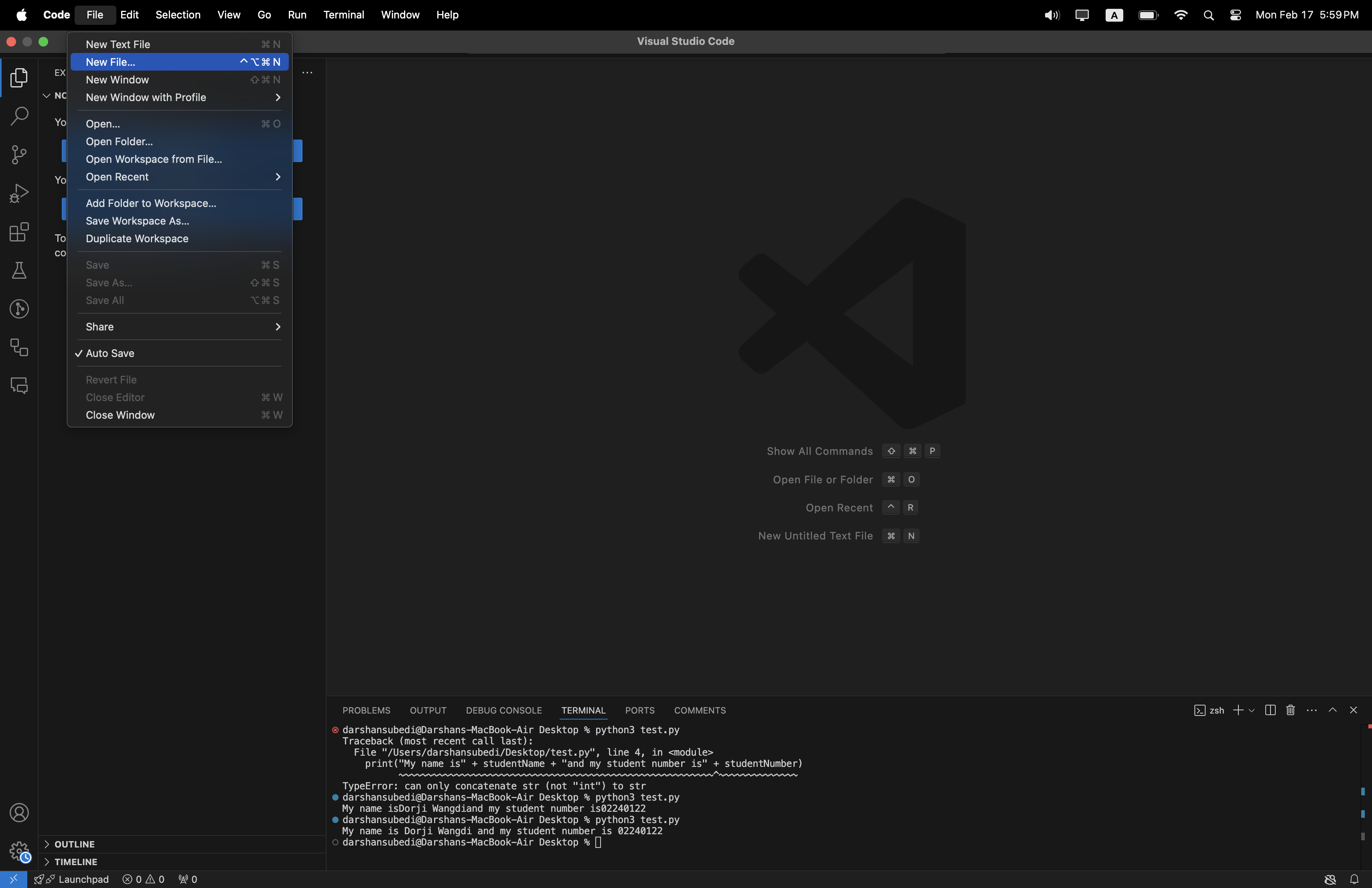
Step 3: In the drop-down menu as shown below, select the Python file option.

Step 4: Type the following simple program that will print your name and student ID:
studentName = "Sonam Choden"
studentNumber = "02240122"
print("My name is " + studentName + " and my student number is " + studentNumber)
Step 5: In the top left-hand corner, select the File tab, click on the Save As tab, and select a destination folder (eg: Desktop). Then save your file with the name practical1.py
Note that your file name must have no spaces and avoid using special characters, you must follow this rule for all files & folders created for your practicals here after
Step 6: Click on the terminal window, and use the ls (list all files) command to locate the folder you previously saved your file in (i.e. Desktop). Use the cd(change directory eg: cd Desktop ) command to access your saved file.
Step 7: Use the python3 command followed by your file name to run your file.
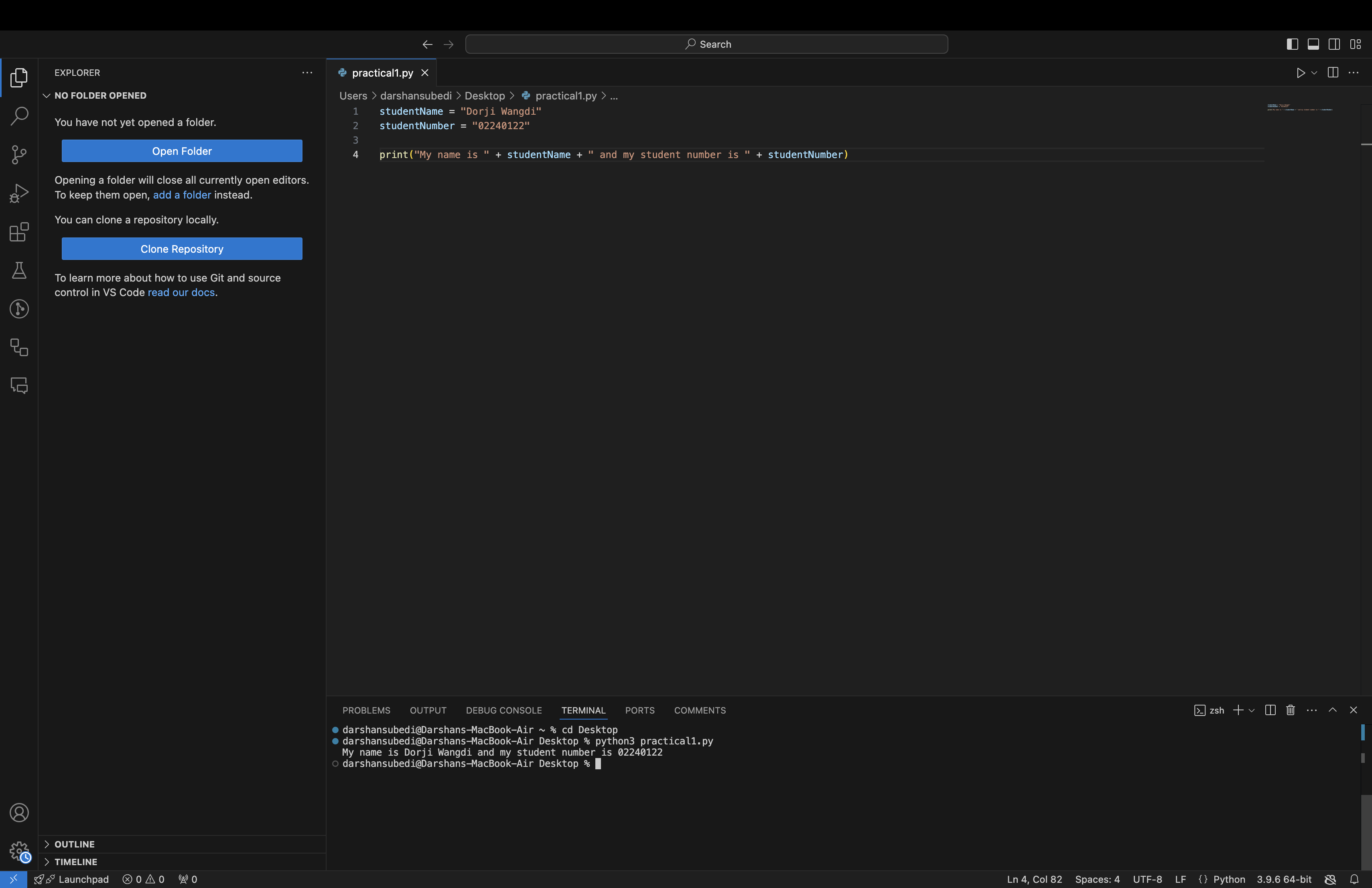
Congratulations, you have completed the first part of your practical. You now know:
- How to create a Python file.
- How to save a Python file.
- How to locate a file in your computer using the ls and cd command in the terminal window.
- How to run your Python file.
Part 2: Git installation
Step 1: Download git on your computer. The steps may vary depending on if you are using a Windows, Mac, or Linux operating system on your computer.
Tutorial for windows: https://www.youtube.com/watch?v=iYkLrXobBbA
Tutorial for Mac: https://www.youtube.com/watch?v=B4qsvQ5IqWk
Note: it is recommended to use a package manager like homebrew for any software you install into your computer here after
Download git from here: https://git-scm.com/downloads
Part 3: Using git
Once you have successfully installed git, open the VScode window you were previously working on. Click on the terminal window.
Step 1: To confirm if git was properly installed in your computer, in the terminal window, type the following command:
git -version
The output must show the current version of git installed on your computer. If there are any errors, it means that git wasn't properly installed on your computer, seek assistance from your module tutor to fix this issue.
Before you proceed to step 2, ensure that the file you created earlier is now saved inside a folder. The folder can be named CSF101Practicals.
Step 2: From the terminal window, ensure that your current directory is the folder you created inside which you have saved for your file. You can verify this by checking your terminal and seeing if the file path is correct:
Example: in the image below, you can see that the last part of my file path reflects the current directory I am accessing using the terminal.
Step 3: Use the following command to initialize a git repository
git init
This initializes an empty git repository inside your folder
Step 4:
Create branch in the repository
git branch -M main
Step 5: Next, type the following command
git add .
This adds all the files that have been changed on created to a staging environment.
Step 6: Next, type the following command
git commit -m "My first commit"
You have now made your very first git commit. To check all commits that were made to your git repository, you can type the following command
git log
A successful repository and commit can be seen as follows:
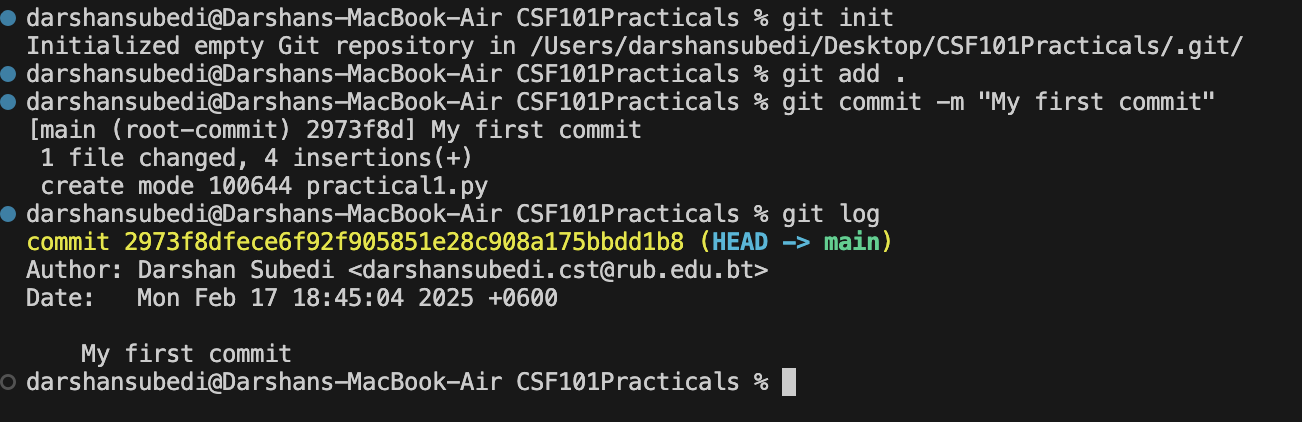
Part 4: Making changes to the file in a git repository
Step 1: Open your VScode window.
Step 2: Make some changes in the file that is saved in your git repository (i.e. Practical1.py ). You can see the changes I have in comparison to my previous code snippet. I have changed the student name and student number variable.
studentName = "Jigme Zangmo"
studentNumber = "02190102"
print("My name is " + studentName + " and my student number is " + studentNumber)
Step 3: go to the terminal and follow Step 4 from Part 3 of this practical as follows.
git add .
Then type the following command:
git status
You can see that git has detected some changes made to your working repository.
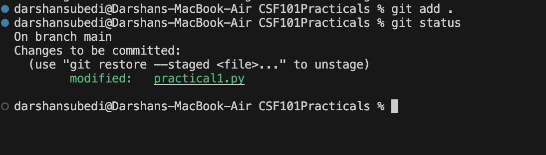
Continue with the following commands:
git commit -m "My Second commit"
Step 5: Using the git log command, you can now see the details of the two separate commits that were made into the repository.
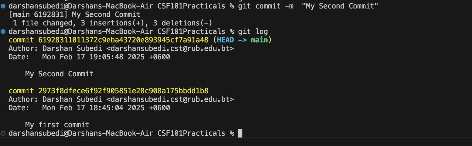
Congratulations you now know how to:
- Initialize a git repository
- Add and commit files to the git repository
- Make changes to the files inside the repository and make new commits
- View the log of all commits made to the repository
Part 5: Using GitHub
Lets start first by creating a repository in github
Step 1: Using a browser, search for github.com and login using your credentials
Step 2: Click on your profile avatar in the top right-hand corner of the screen, select the repository option in the drop-down menu
Step 3: Click on the new option on the top right-hand side of the screen. In the create repository page, name your new repository in the format shown below. Select your account as the repository owner and click on the Create Repository button on the bottom right side of the page:
Eg: 02240224_CSF101_Practicals


Step 4: Once a empty repository is created as shown below, click on the SSH option and copy the link as highlighted below:

Step 5: Go back to the terminal of your VScode window and paste this link there. Once you have entered the command, you can type git remote -v to check if the repository has been added successfully:
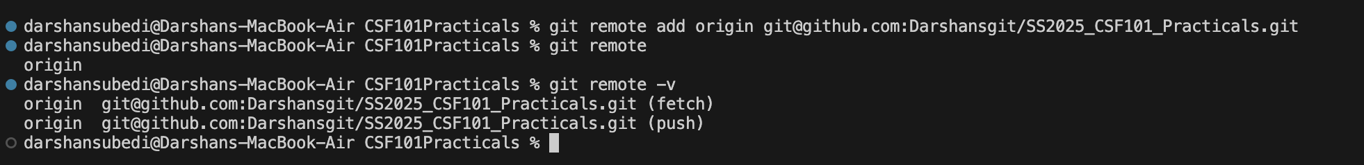
Note: the following step is very important
Step 6: Navigate to the same drop-down menu as shown in Step 2 and click on the settings option. Navigate the settings page and select the developer options
Step 7: Click on the Tokens (classic) option on the left-hand side and select the generate new token(classic) option.
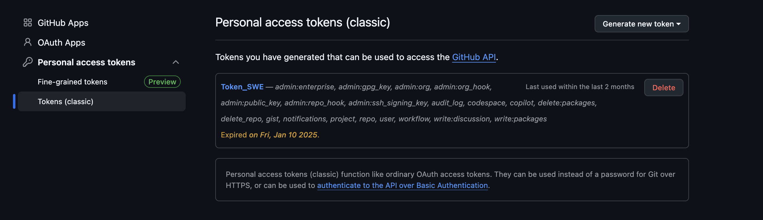
Step 8: In the generate token page, provide a small note for the token, and in the Expiration drop-down menu, select the no expiration option. Then select all the checkboxes on this page and click on the generate token button at the bottom of the page

Step 9: Copy the token link that has been generated and save it in any application on your desktop. This token is important and will not be visible again.
Step 10: Take your token and replace it with the following command:
git remote set-url origin https://<token>@github.com/<username>/<repo>
Where:
- token - token you just generated in GitHub
- username - your GitHub username
- repo - the name of your GitHub repo
Your command should look like this:
git remote set-url origin https://ghp_OBJnrsdfsdaP251jFasdfasde4ObzzAw1qc1tA@github.com/Darshansgit/02190108_CSF101_Practicals
Step 11: Finally you can type the following command in your terminal:
git push -u origin main
If your push was successful, you will see the following output.
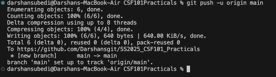
You can now go and check your empty GitHub repository and notice that the file that you had created on your computers local repository is now on git.
Note: for future pushes, you need not follow Step 6 to Step 10. The GitHub personal access token generation is a one-time thing (once for each repo) and you do not need to generate a new key for every push. Once you are done committing your code locally using git, you may proceed with the git push -u origin main command to directly push your code to git here after.
Congratulations, you now know how to:
- Create an empty GitHub repository
- Generate an access token for you to push your local repository into the remote repository on GitHub
- Authenticate using the access token (this needs to be done one time only)
- Push your local repository to your remote repository.
This concludes Practical 0. Hereafter, all your practicals are expected to be completed and pushed to Git Hub. Your GitHub repository will be reviewed before the end of the semester to check if you have completed all your practicals. Please practice this process to get familiar with git and github.
Practical 1: Python Basics
Python Comments
This is done with the # character at the beginning of the line
# This is a comment line in the code
Creating a Function
In Python a function is defined using the def keyword:
def my_function():
print("Hello from a function")
# Calling the function
my_function()
Scope
Notice how s has different defined value for the string in local scope within the function func() versus global scope for the overall python file.
def func():
# Local scope
s = "Me too! (on local scope)"
print(s)
# Global scope
s = "I love python! (on global scope)"
print(s)
Basic Data Types - Integer, Float, Boolean, None and Type Casting
# Integer
pi = 3.14
pi2 = int(pi)
print(pi)
print(pi2)
# Float
pi3 = "3.14"
print(type(pi3))
pi4 = float(pi3)
print(type(pi4))
# Boolean
print(0<1)
print(1>0)
bool(0)
bool(1)
bool("Hello")
# None
x = None
print(x)
Basic Data Types: String and Manipulations
print("Hello!!!!")
print("This is my first script!")
a = """Lorem ipsum dolor sit amet,
consectetur adipiscing elit,
sed do eiusmod tempor incididunt
ut labore et dolore magna aliqua."""
print(a)
# String functions
print(len(a))
print(a.upper())
print(a.lower())
print(a.count('i'))
print(a.find('d'))
print(a.split())
# String Concatenation
b = "Hello"
c = "Hello"
d = b + "!!" + c + "??"
print(d)
# String replication
print("Alice" * 5)
# String formatting
name = "Karma"
print(f"Hello {name}")
print("Greeting to you, {}".format(name))
Number = 2
print("There are %d %s in the class" %(Number, name))
Basic Data Structures
# List
thislist = ["apple", "banana", "cherry"]
print(thislist)
print(len(thislist))
print(thislist.index("banana"))
thislist.remove("banana")
thislist.insert(1, "strawberry")
print(thislist)
# Tuple
thistuple = ("apple", "banana", "cherry")
print(thistuple)
print(len(thistuple))
print(type(thistuple))
# Set
thisset = {"apple", "banana", "cherry", True, 1, 2}
print(thisset)
print(len(thisset))
print(type(myset))
# Dictionary
thisdict = {
"brand": "Ford",
"model": "Mustang",
"year": 1964
}
print(thisdict)
print(thisdict["brand"])
Class excercise:
Q1. Array manipulation:
Refer to the following documentation on python list methods Link
Create a python list and name it first_list as shown below:
first_list = [0,1,2,3,4,5,6,7,8,9]
Create a second empty list named inverse_list:
inverse_list = []
Using the
.append()
.pop()
methods, create the implementation of a stack whereby you de-que elements from the first list and enqueee them into the second list. Your output must be as follows:
inverse_list = [9,8,7,6,5,4,3,2,1,0]
Sample scaffold (fill up with logic and code where necesarry):
first_list = [0,1,2,3,4,5,6,7,8,9]
inverse_list = [9,8,7,6,5,4,3,2,1,0]
index = 9
#Hint, use a while loop to loop throught first list from the last index
while index < :
inverse_list.append()
index =
print(inverse_list)
Q2. Implementing Functions
Take your array invers implementation from question 1 and define a function known as reverse_array. Pass the
first_list() as an argument into the array and ensure that inverse_list is returned when the function is called.
def reverse_array(first_list):
#logic and code from Q1
reverse_array(first_list)
Practical 2: Coding Basic Functions
Objective
In this lab, you will create a Python program that analyzes a text file and calculates various statistics using control structures. This exercise will help you practice file handling, string manipulation, and using loops and conditionals in Python.
Prerequisites
- Basic knowledge of Python syntax
- Understanding of file operations
Lab Steps
Step 0: Preparation
Create a folder and name it practical4. Download the sample.txt text file from this link and save it inside the folder. Create your practical5.py file in the same folder and continue with the subsequent steps.
Step 1: Open and Read a Text File
First, let's create a function to open and read a text file:
def read_file(filename):
with open(filename, 'r') as file:
return file.read()
# Test the function
content = read_file('sample.txt')
print(content[:100]) # Print the first 100 characters
Step 2: Count the Number of Lines
Now, let's count the number of lines in the file:
def count_lines(content):
return len(content.split('\n'))
# Test the function
num_lines = count_lines(content)
print(f"Number of lines: {num_lines}")
Step 3: Count Words
Next, we'll count the total number of words in the file:
def count_words(content):
return len(content.split())
# Test the function
num_words = count_words(content)
print(f"Number of words: {num_words}")
Step 4: Find the Most Common Word
Let's find the most common word in the text:
from collections import Counter
def most_common_word(content):
words = content.lower().split()
word_counts = Counter(words)
return word_counts.most_common(1)[0]
# Test the function
common_word, count = most_common_word(content)
print(f"Most common word: '{common_word}' (appears {count} times)")
Step 5: Calculate Average Word Length
Now, let's calculate the average word length:
def average_word_length(content):
words = content.split()
total_length = sum(len(word) for word in words)
return total_length / len(words)
# Test the function
avg_length = average_word_length(content)
print(f"Average word length: {avg_length:.2f} characters")
Step 6: Combine Everything into a Main Function
Finally, let's combine all these functions into a main function that analyzes the text file:
def analyze_text(filename):
content = read_file(filename)
num_lines = count_lines(content)
num_words = count_words(content)
common_word, count = most_common_word(content)
avg_length = average_word_length(content)
print(f"File: {filename}")
print(f"Number of lines: {num_lines}")
print(f"Number of words: {num_words}")
print(f"Most common word: '{common_word}' (appears {count} times)")
print(f"Average word length: {avg_length:.2f} characters")
# Run the analysis
analyze_text('sample.txt')
Exercises for Students
- Modify the program to count the number of unique words in the text.
- Add a function to find the longest word in the text.
- Implement a feature to count the occurrences of a specific word (case-insensitive).
- Create a function to calculate the percentage of words that are longer than the average word length.
Conclusion
In this lab, you've created a text file analyzer using Python. You've practiced file handling, string manipulation, and using control structures like loops and conditionals. The modular approach we've taken allows for easy expansion and modification of the program.
Remember to test your code with different text files to ensure it works correctly in various scenarios.
Practical 3: Practicing Python Loops and Logical Conditions
Objective
In this lab, you will implement both recursive and iterative approaches to generate Fibonacci sequences in Python. This exercise will help you understand the differences between recursive and iterative problem-solving techniques, as well as analyze their performance characteristics.
Prerequisites
- Basic knowledge of Python syntax
- Understanding of functions in Python
- Familiarity with recursion and iteration concepts
Lab Steps
Step 1: Python Operators
Looking into python operators with print statements
import random
a = 10
b = random.randint(0,20)
c = 100
print("a is", a, "and", "b is", b)
print("The answer to a + b is", a + b)
print("a < b is", a < b)
print("a == b is", a == b)
print("a + b is", a + b)
print("a * b is", a * b)
print("a to the power of b is", a ** b)
Step 2: If-Else Statements
Trying out if, elif and else
a = 33
b = 200
if b > a:
print("b is greater than a")
a = 33
b = 33
if b > a:
print("b is greater than a")
elif a == b:
print("a and b are equal")
a = 200
b = 33
if b > a:
print("b is greater than a")
elif a == b:
print("a and b are equal")
else:
print("a is greater than b")
Step 3: Match case Statements
Printing different days
def main():
day = 8
match day:
case 1:
print("Monday")
case 2:
print("Tuesday")
case 3:
print("Wednesday")
case 4:
print("Thursday")
case 5:
print("Friday")
case 6:
print("Saturday")
case 7:
print("Sunday")
case _:
print("Not a weekday")
main()
Step 4: While Loops
While Loop
A guessing game using a while loop
import random
a = 10
b = random.randint(0,20)
while(c != b):
c = int(input("Enter Guess! "))
if (c == b):
print("You won!")
break
else:
print("Wrong Answer, Try Again!")
Remember to analyze the time and space complexity of each approach and consider how they might perform with very large inputs.
Practical 4: Flow Chart and Pseudo Code
Objective
In this lab, you will implement following Exercises. This exercise will help you understand the flow chart and pseudo code principles.
Submission Date:
Prerequisites
- Basic knowledge of Python syntax
Lab Steps
Step 1: Download and install Flowgorithm
Get Flowgorithm from the following link
http://www.flowgorithm.org/download/index.html
Step 2: Follow Basic Tutorial
Check the beginner video about checking a number for even or odd property.
Step 3: Implement Basic Sum
Implement the following flow chart, and create python source code
Step 4: Implement Largest Number
Implement the following flow chart, and create python source code
Step 5: Study Pseudo Code
Binary search is a searching algorithm that works only for sorted search space. It repeatedly divides the search space into half by using the fact that the search space is sorted and checking if the desired search result will be found in the left or right half. Example: Given a sorted array Arr[] and a value X, The task is to find the index at which X is present in Arr[]. Below is the pseudocode for Binary search.
BinarySearch(ARR, X, LOW, HIGH)
repeat till LOW = HIGH
MID = (LOW + HIGH)/2
if (X == ARR[mid])
return MID
else if (x > ARR[MID])
LOW = MID + 1
else
HIGH = MID – 1
Step 6: Try past midterm question
Design a simple weather data analysis program for a local meteorology station. The program should calculate the average temperature, convert units, and determine temperature ranges.
Create a flowchart and write pseudocode for this system with the following requirements:
- Ask the user to input the highest and lowest temperatures for a day (in Celsius).
- Calculate and display the average temperature for the day.
- Convert the average temperature to Fahrenheit and display it.
Determine and display the temperature range category based on the following criteria:
- If the range (difference between highest and lowest) is less than 10°C: "Stable"
- If the range is between 10°C and 20°C: "Moderate"
- If the range is greater than 20°C: "Volatile"
- If either input temperature is less than -50°C or greater than 50°C, display an error message for invalid input.
Exercises for Students
- Implement more complex algorithms in flowgorithm
- Create Pseudo Code for these two simple algorithms
Conclusion
In this lab, you've learned flow charts and on looking at pseudo code
Key takeaways:
Practical 5: Implementing Linear and Binary Search Algorithms
Objective
In this lab, you will implement both linear and binary search algorithms in Python. You'll learn about the differences between these search methods, their time complexities, and when to use each one. This exercise will help you practice algorithm implementation, list manipulation, and control structures in Python.
Submission Date: October 29th
Prerequisites
- Basic knowledge of Python syntax
- Understanding of lists and functions in Python
- Familiarity with control structures (if statements, loops)
Lab Steps
Step 1: Implement Linear Search
Let's start by implementing the linear search algorithm:
def linear_search(arr, target):
for i in range(len(arr)):
if arr[i] == target:
return i # Return the index if the target is found
return -1 # Return -1 if the target is not in the list
# Test the function
test_list = [3, 1, 4, 1, 5, 9, 2, 6, 5, 3, 5]
result = linear_search(test_list, 6)
print(f"Linear Search: Index of 6 is {result}")
Step 2: Implement Binary Search
Now, let's implement the binary search algorithm. Remember, binary search requires a sorted list:
def binary_search(arr, target):
left, right = 0, len(arr) - 1
while left <= right:
mid = (left + right) // 2
if arr[mid] == target:
return mid # Return the index if the target is found
elif arr[mid] < target:
left = mid + 1
else:
right = mid - 1
return -1 # Return -1 if the target is not in the list
# Test the function
test_list_sorted = sorted(test_list)
result = binary_search(test_list_sorted, 6)
print(f"Binary Search: Index of 6 in sorted list is {result}")
Step 3: Compare Performance
Let's create a function to compare the performance of both search algorithms:
import time
def compare_search_algorithms(arr, target):
# Linear Search
start_time = time.time()
linear_result = linear_search(arr, target)
linear_time = time.time() - start_time
# Binary Search (on sorted array)
arr_sorted = sorted(arr)
start_time = time.time()
binary_result = binary_search(arr_sorted, target)
binary_time = time.time() - start_time
print(f"Linear Search: Found at index {linear_result}, Time: {linear_time:.6f} seconds")
print(f"Binary Search: Found at index {binary_result}, Time: {binary_time:.6f} seconds")
# Test with a larger list
large_list = list(range(10000))
compare_search_algorithms(large_list, 8888)
Step 4: Implement Recursive Binary Search
Let's also implement a recursive version of binary search:
def binary_search_recursive(arr, target, left, right):
if left > right:
return -1
mid = (left + right) // 2
if arr[mid] == target:
return mid
elif arr[mid] < target:
return binary_search_recursive(arr, target, mid + 1, right)
else:
return binary_search_recursive(arr, target, left, mid - 1)
# Test the recursive function
result = binary_search_recursive(test_list_sorted, 6, 0, len(test_list_sorted) - 1)
print(f"Recursive Binary Search: Index of 6 in sorted list is {result}")
Step 5: Create a Main Function
Finally, let's create a main function that demonstrates all our search algorithms:
def main():
# Create a list of 20 random integers between 1 and 100
import random
test_list = [random.randint(1, 100) for _ in range(20)]
print("Original list:", test_list)
print("Sorted list:", sorted(test_list))
target = random.choice(test_list) # Choose a random target from the list
print(f"\nSearching for: {target}")
# Linear Search
result = linear_search(test_list, target)
print(f"Linear Search: Found at index {result}")
# Binary Search (iterative)
sorted_list = sorted(test_list)
result = binary_search(sorted_list, target)
print(f"Binary Search (iterative): Found at index {result}")
# Binary Search (recursive)
result = binary_search_recursive(sorted_list, target, 0, len(sorted_list) - 1)
print(f"Binary Search (recursive): Found at index {result}")
# Compare performance
print("\nPerformance Comparison:")
compare_search_algorithms(list(range(100000)), 99999)
if __name__ == "__main__":
main()
Exercises for Students
- Modify the linear search function to return all indices where the target appears, not just the first one.
- Implement a function that uses binary search to find the insertion point for a target value in a sorted list.
- Create a function that counts the number of comparisons made in each search algorithm.
- Implement a jump search algorithm and compare its performance with linear and binary search.
Conclusion
In this lab, you've implemented both linear and binary search algorithms in Python. You've learned about their differences, time complexities, and when to use each one. The modular approach we've taken allows for easy testing and comparison of these algorithms.
Remember that while binary search is generally faster for large sorted lists, it requires the list to be sorted first. Linear search, although slower for large lists, works on unsorted lists and can be more efficient for small lists or when searching for multiple occurrences of an element.
Practical 6: Implementing Sorting Algorithms
Objective
In this lab, you will implement three classic sorting algorithms: Bubble Sort, Merge Sort, and Quick Sort. This exercise will help you understand the mechanics of these algorithms and compare their performance.
Submission Date: November 4st
Prerequisites
- Basic knowledge of Python syntax
- Understanding of lists and functions in Python
- Familiarity with time complexity concepts (optional, but helpful)
Lab Steps
Step 1: Implement Bubble Sort
Bubble Sort is a simple sorting algorithm that repeatedly steps through the list, compares adjacent elements and swaps them if they are in the wrong order.
def bubble_sort(arr):
n = len(arr)
for i in range(n):
for j in range(0, n - i - 1):
if arr[j] > arr[j + 1]:
arr[j], arr[j + 1] = arr[j + 1], arr[j]
return arr
# Test the function
test_arr = [64, 34, 25, 12, 22, 11, 90]
sorted_arr = bubble_sort(test_arr.copy())
print("Bubble Sort Result:", sorted_arr)
Step 2: Implement Merge Sort
Merge Sort is a divide-and-conquer algorithm that divides the input array into two halves, recursively sorts them, and then merges the two sorted halves.
def merge_sort(arr):
if len(arr) <= 1:
return arr
mid = len(arr) // 2
left = merge_sort(arr[:mid])
right = merge_sort(arr[mid:])
return merge(left, right)
def merge(left, right):
result = []
i, j = 0, 0
while i < len(left) and j < len(right):
if left[i] <= right[j]:
result.append(left[i])
i += 1
else:
result.append(right[j])
j += 1
result.extend(left[i:])
result.extend(right[j:])
return result
# Test the function
test_arr = [64, 34, 25, 12, 22, 11, 90]
sorted_arr = merge_sort(test_arr)
print("Merge Sort Result:", sorted_arr)
Step 3: Implement Quick Sort
Quick Sort is another divide-and-conquer algorithm that picks an element as a pivot and partitions the array around the pivot.
def quick_sort(arr):
if len(arr) <= 1:
return arr
else:
pivot = arr[0]
less = [x for x in arr[1:] if x <= pivot]
greater = [x for x in arr[1:] if x > pivot]
return quick_sort(less) + [pivot] + quick_sort(greater)
# Test the function
test_arr = [64, 34, 25, 12, 22, 11, 90]
sorted_arr = quick_sort(test_arr)
print("Quick Sort Result:", sorted_arr)
Step 4: Compare Performance
Now, let's create a function to compare the performance of these sorting algorithms:
import time
import random
def compare_sorting_algorithms(arr):
algorithms = [
("Bubble Sort", bubble_sort),
("Merge Sort", merge_sort),
("Quick Sort", quick_sort)
]
for name, func in algorithms:
arr_copy = arr.copy()
start_time = time.time()
func(arr_copy)
end_time = time.time()
print(f"{name} took {end_time - start_time:.6f} seconds")
# Generate a large random array
large_arr = [random.randint(1, 1000) for _ in range(1000)]
# Compare the algorithms
compare_sorting_algorithms(large_arr)
Exercises for Students
- Implement an in-place version of Quick Sort to improve its space efficiency.
- Modify Bubble Sort to stop early if the list becomes sorted before all passes are complete.
- Implement a hybrid sorting algorithm that uses Insertion Sort for small subarrays in Merge Sort or Quick Sort.
- Create a visualization of how each sorting algorithm works using a library like Matplotlib.
Conclusion
In this lab, you've implemented three classic sorting algorithms: Bubble Sort, Merge Sort, and Quick Sort. You've also compared their performance on a large random array.
Key takeaways:
- Bubble Sort is simple but inefficient for large datasets (O(n^2) time complexity).
- Merge Sort provides stable, predictable performance (O(n log n) time complexity) but requires extra space.
- Quick Sort is often the fastest in practice (average O(n log n) time complexity) but can degrade to O(n^2) in worst cases.
Remember that the choice of sorting algorithm depends on the specific requirements of your application, such as the size and initial order of the data, memory constraints, and whether a stable sort is needed.
Practical 7: Algorithms Exercises on Arrays, Hashing, Two Pointers, Sliding Window
Objective
In this lab, you will implement following algorithms: Valid Anagram, Two Sums, Valid Palindrome, Three Sums, Sliding Window Exercises. This exercise will help you understand the mechanics of these algorithms and compare their performance.
Submission Date: November 4st
Prerequisites
- Basic knowledge of Python syntax
- Understanding of lists and functions in Python
- Familiarity with time complexity concepts (optional, but helpful)
Lab Steps: Algorithm Problems on Contains Duplicate, Valid Anagram, Two Sums
Leetcode problems on Contains Duplicate, Valid Anagram, Two Sums
Step 1: Contains Duplicate
https://leetcode.com/problems/contains-duplicate
Given an integer array nums, return true if any value appears at least twice in the array, and return false if every element is distinct.
Example:
Input: nums = [1,2,3,1]
Output: true
Explanation: The element 1 occurs at the indices 0 and 3.
Input: nums = [1,2,3,4]
Output: false
Explanation: All elements are distinct.
Python
class Solution:
def containsDuplicate(self, nums):
return len(set(nums))!=len(nums)
Python 3
class Solution:
def containsDuplicate(self, nums: List[int]) -> bool:
return len(set(nums))!=len(nums)
HashSet Method
# Python Program check if there are any duplicates
# in the array using Hashing
def checkDuplicates(arr):
n = len(arr)
# Create a set to store the unique elements
st = set()
# Iterate through each element
for i in range(n):
# If the element is already present, return true
# Else insert the element into the set
if arr[i] in st:
return True
else:
st.add(arr[i])
# If no duplicates are found, return false
return False
if __name__ == "__main__":
arr = [4, 5, 6, 4]
print(checkDuplicates(arr))
Step 2: Valid Anagram
https://leetcode.com/problems/valid-anagram
Given two strings s and t, return true if t is an anagram of s, and false otherwise. Anagram is a word, phrase, or name formed by rearranging the letters of another.
Example:
Input: s = "anagram", t = "nagaram"
Output: true
Input: s = "rat", t = "car"
Output: false
Python
class Solution:
def isAnagram(self, s, t):
if len(s) != len(t):
return False
count = [0] * 26
for i in range(len(s)):
count[ord(s[i]) - ord('a')] += 1
count[ord(t[i]) - ord('a')] -= 1
return (len(set(count)) == 1 and list(set(count))[0] == 0)
Python 3
class Solution:
def isAnagram(self, s: str, t: str) -> bool:
if len(s) != len(t):
return False
count = [0] * 26
for i in range(len(s)):
count[ord(s[i]) - ord('a')] += 1
count[ord(t[i]) - ord('a')] -= 1
return (len(set(count)) == 1 and list(set(count))[0] == 0)
Using Hash Map or Dictionary
# Python Code to check if two Strings are anagram of
# each other using Dictionary
def areAnagrams(s1, s2):
# Create a hashmap to store character frequencies
charCount = {}
# Count frequency of each character in string s1
for ch in s1:
charCount[ch] = charCount.get(ch, 0) + 1
# Count frequency of each character in string s2
for ch in s2:
charCount[ch] = charCount.get(ch, 0) - 1
# Check if all frequencies are zero
for value in charCount.values():
if value != 0:
return False
# If all conditions satisfied, they are anagrams
return True
if __name__ == "__main__":
s1 = "geeks"
s2 = "kseeg"
print("true" if areAnagrams(s1, s2) else "false")
Step 3: Two Sum
https://leetcode.com/problems/two-sum
Given an array of integers nums and an integer target, return indices of the two numbers such that they add up to target. You may assume that each input would have exactly one solution, and you may not use the same element twice. You can return the answer in any order.
Example:
Input: nums = [2,7,11,15], target = 9
Output: [0,1]
Explanation: Because nums[0] + nums[1] == 9, we return [0, 1].
Input: nums = [3,2,4], target = 6
Output: [1,2]
Python3
class Solution:
def twoSum(self, nums: list[int], target: int) -> list[int]:
for i in range(1, len(nums)):
for j in range(i, len(nums)):
if nums[j] + nums[j - i] == target:
return [j, j - i]
return []
Python
class Solution:
def twoSum(self, nums, target):
for i in range(1, len(nums)):
for j in range(i, len(nums)):
if nums[j] + nums[j - i] == target:
return [j, j - i]
return []
One-Pass Hash Table Method
class Solution(object):
def twoSum(self, nums, target):
numMap = {}
for i, num in enumerate(nums):
complement = target - num
if complement in numMap:
return [numMap[complement], i]
numMap[num] = i
return []
Algorithm Problems on Valid Palindrome, Three Sums
Leetcode problems on Valid Palindrome, Three Sums
Step 4: Valid Palindrome
https://leetcode.com/problems/valid-palindrome
A phrase is a palindrome if, after converting all uppercase letters into lowercase letters and removing all non-alphanumeric characters, it reads the same forward and backward. Alphanumeric characters include letters and numbers. Given a string s, return true if it is a palindrome, or false otherwise.
Example:
Input: s = "A man, a plan, a canal: Panama"
Output: true
Explanation: "amanaplanacanalpanama" is a palindrome.
Input: s = "race a car"
Output: false
Explanation: "raceacar" is not a palindrome.
Python 3
class Solution:
def isPalindrome(self, s: str) -> bool:
s = [c.lower() for c in s if c.isalnum()]
return all (s[i] == s[~i] for i in range(len(s)//2))
Python
class Solution:
def isPalindrome(self, s):
s = [c.lower() for c in s if c.isalnum()]
return all (s[i] == s[~i] for i in range(len(s)//2))
Step 5: Three Sum
https://leetcode.com/problems/3sum
Given an integer array nums, return all the triplets [nums[i], nums[j], nums[k]] such that i != j, i != k, and j != k, and nums[i] + nums[j] + nums[k] == 0. Notice that the solution set must not contain duplicate triplets.
Example:
Input: nums = [-1,0,1,2,-1,-4]
Output: [[-1,-1,2],[-1,0,1]]
Explanation:
nums[0] + nums[1] + nums[2] = (-1) + 0 + 1 = 0.
nums[1] + nums[2] + nums[4] = 0 + 1 + (-1) = 0.
nums[0] + nums[3] + nums[4] = (-1) + 2 + (-1) = 0.
The distinct triplets are [-1,0,1] and [-1,-1,2].
Notice that the order of the output and the order of the triplets does not matter.
Input: nums = [0,1,1]
Output: []
Explanation: The only possible triplet does not sum up to 0.
Python 3
class Solution:
def threeSum(self, nums: List[int]) -> List[List[int]]:
target = 0
nums.sort()
s = set()
output = []
for i in range(len(nums)):
j = i + 1
k = len(nums) - 1
while j < k:
sum = nums[i] + nums[j] + nums[k]
if sum == target:
s.add((nums[i], nums[j], nums[k]))
j += 1
k -= 1
elif sum < target:
j += 1
else:
k -= 1
output = list(s)
return output
Python
class Solution:
def threeSum(self, nums):
target = 0
nums.sort()
s = set()
output = []
for i in range(len(nums)):
j = i + 1
k = len(nums) - 1
while j < k:
sum = nums[i] + nums[j] + nums[k]
if sum == target:
s.add((nums[i], nums[j], nums[k]))
j += 1
k -= 1
elif sum < target:
j += 1
else:
k -= 1
output = list(s)
return output
Algorithm Problems on Sliding Window (Best Time to Buy And Sell Stock), Longest Substring Without Repeating Characters
Leetcode problems on Sliding Window (Best Time to Buy And Sell Stock), Longest Substring Without Repeating Characters
Step 6: Best Time to Buy And Sell Stock
https://leetcode.com/problems/best-time-to-buy-and-sell-stock
You are given an array prices where prices[i] is the price of a given stock on the ith day. You want to maximize your profit by choosing a single day to buy one stock and choosing a different day in the future to sell that stock. Return the maximum profit you can achieve from this transaction. If you cannot achieve any profit, return 0.
Example:
Input: prices = [7,1,5,3,6,4]
Output: 5
Explanation: Buy on day 2 (price = 1) and sell on day 5 (price = 6), profit = 6-1 = 5. Note that buying on day 2 and selling on day 1 is not allowed because you must buy before you sell.
Python
class Solution:
def maxProfit(self, prices):
buy = prices[0]
profit = 0
for i in range(1, len(prices)):
if prices[i] < buy:
buy = prices[i]
elif prices[i] - buy > profit:
profit = prices[i] - buy
return profit
Step 7: Longest Substring Without Repeating Characters
https://leetcode.com/problems/longest-substring-without-repeating-characters
Given a string s, find the length of the longest without duplicate characters.
Example:
Input: s = "abcabcbb”
Output: 3
Explanation: The answer is "abc", with the length of 3.
Input: s = "bbbbb"
Output: 1
Explanation: The answer is "b", with the length of 1.
class Solution:
def lengthOfLongestSubstring(self, s):
n = len(s)
maxLength = 0
charSet = set()
left = 0
for right in range(n):
if s[right] not in charSet:
charSet.add(s[right])
maxLength = max(maxLength, right - left + 1)
else:
while s[right] in charSet:
charSet.remove(s[left])
left += 1
charSet.add(s[right])
return maxLength
Exercises for Students
Conclusion
In this lab, you've implemented some algorithms: Contains Duplicate, Valid Anagram, Two Sums, Valid Palindrome, Three Sums and Sliding Window Exercises.
Key takeaways:
- How to create algorithms that solve specific problems.
Practical 8: Implementing Stacks and Queues, including leetcode problems to Implement Stack using Queue(s), and Valid Parentheses
Objective
In this lab, you will implement stack and queue data structures in Python and use them to solve practical problems. This exercise will help you understand these fundamental data structures and their applications.
Submission Date: October 29th
Prerequisites
- Basic knowledge of Python syntax
- Understanding of lists in Python
- Familiarity with classes in Python (optional, but helpful)
Part 1: Implementing a Stack
A stack is a Last-In-First-Out (LIFO) data structure. Let's implement a basic stack class:
class Stack:
def __init__(self):
self.items = []
def is_empty(self):
return len(self.items) == 0
def push(self, item):
self.items.append(item)
def pop(self):
if not self.is_empty():
return self.items.pop()
else:
raise IndexError("Stack is empty")
def peek(self):
if not self.is_empty():
return self.items[-1]
else:
raise IndexError("Stack is empty")
def size(self):
return len(self.items)
# Test the Stack
stack = Stack()
stack.push(1)
stack.push(2)
stack.push(3)
print(stack.pop()) # Should print 3
print(stack.peek()) # Should print 2
print(stack.size()) # Should print 2
Part 2: Implementing a Queue
A queue is a First-In-First-Out (FIFO) data structure. Let's implement a basic queue class:
class Queue:
def __init__(self):
self.items = []
def is_empty(self):
return len(self.items) == 0
def enqueue(self, item):
self.items.append(item)
def dequeue(self):
if not self.is_empty():
return self.items.pop(0)
else:
raise IndexError("Queue is empty")
def front(self):
if not self.is_empty():
return self.items[0]
else:
raise IndexError("Queue is empty")
def size(self):
return len(self.items)
# Test the Queue
queue = Queue()
queue.enqueue(1)
queue.enqueue(2)
queue.enqueue(3)
print(queue.dequeue()) # Should print 1
print(queue.front()) # Should print 2
print(queue.size()) # Should print 2
Part 3: Leetcode Lesson: Implementing Stack Using Queue
1. Problem Statement
Implement a last-in-first-out (LIFO) stack using only two queues. The implemented stack should support all the functions of a normal stack (push, pop, top, empty).
Implement the MyStack class:
push(x)Pushes element x to the top of the stack.pop()Removes the element on the top of the stack and returns it.top()Returns the element on the top of the stack.empty()Returnstrueif the stack is empty,falseotherwise.
Notes:
- You must use only standard queue operations, which means only
push to back,peek/pop from front,size, andis emptyare valid. - Depending on your language, the queue may not be supported natively. You may simulate a queue using a list or deque (double-ended queue), as long as you use only a queue's standard operations.
2. Conceptual Understanding
This problem challenges us to implement a stack (LIFO - Last In, First Out) data structure using only queue (FIFO - First In, First Out) operations. It's like trying to create a stack of plates (where you add and remove from the top) using only queues (where you add to the back and remove from the front).
The key is to find a way to reverse the order of elements when needed, as stacks and queues have opposite ordering principles.
Here's how we can implement the stack using two queues:
- Use two queues:
q1andq2. - For
pushoperation:- Add the new element to
q2. - Move all elements from
q1toq2. - Swap
q1andq2.
- Add the new element to
- For
pop,top, andemptyoperations:- Perform these operations directly on
q1.
- Perform these operations directly on
This approach ensures that q1 always has the elements in the correct stack order (newest on top).
3. Python Implementation
from queue import Queue
class MyStack:
def __init__(self):
self.q1 = Queue()
self.q2 = Queue()
def push(self, x: int) -> None:
self.q2.put(x)
while not self.q1.empty():
self.q2.put(self.q1.get())
self.q1, self.q2 = self.q2, self.q1
def pop(self) -> int:
return self.q1.get()
def top(self) -> int:
return self.q1.queue[0]
def empty(self) -> bool:
return self.q1.empty()
- We use Python's
Queueclass for our queues. pushadds the new element toq2, moves all elements fromq1toq2, then swapsq1andq2.popandtopoperate directly onq1.emptychecks ifq1is empty.
Solving Practical Problems: Now that we have implemented our stack and queue, let's use them to solve some practical problems.
Part 4 Problem: Reverse a String
Use a stack to reverse a string:
def reverse_string(s):
stack = Stack()
for char in s:
stack.push(char)
reversed_string = ""
while not stack.is_empty():
reversed_string += stack.pop()
return reversed_string
# Test the function
print(reverse_string("Hello, World!")) # Should print "!dlroW ,olleH"
Part 5 Problem: Hot Potato Simulation
Use a queue to simulate the Hot Potato game:
def hot_potato(names, num):
queue = Queue()
for name in names:
queue.enqueue(name)
while queue.size() > 1:
for _ in range(num):
queue.enqueue(queue.dequeue())
queue.dequeue()
return queue.dequeue()
# Test the function
names = ["Bill", "David", "Susan", "Jane", "Kent", "Brad"]
print(hot_potato(names, 7)) # The winner's name will be printed
Part 6 Problem: Balanced Parentheses
Use a stack to check if a string of parentheses is balanced:
def is_balanced(parentheses):
stack = Stack()
for p in parentheses:
if p == '(':
stack.push(p)
elif p == ')':
if stack.is_empty():
return False
stack.pop()
return stack.is_empty()
# Test the function
print(is_balanced("((()))")) # Should print True
print(is_balanced("(()")) # Should print False
Part 7 Leetcode Lesson: Valid Parentheses
1. Problem Statement
Given a string s containing just the characters '(', ')', '{', '}', '[' and ']', determine if the input string is valid.
An input string is valid if:
- Open brackets must be closed by the same type of brackets.
- Open brackets must be closed in the correct order.
- Every close bracket has a corresponding open bracket of the same type.
Example 1:
Input: s = "()"
Output: true
Example 2:
Input: s = "()[]{}"
Output: true
Example 3:
Input: s = "(]"
Output: false
Constraints:
- 1 <= s.length <= 10^4
sconsists of parentheses only'()[]{}'
2. Conceptual Understanding
This problem is about validating the structure of nested parentheses. It's similar to checking if HTML tags or code blocks are properly nested and closed.
Think of it like nesting dolls: each smaller doll (inner parenthesis) needs to be completely enclosed by its larger doll (outer parenthesis) of the same type.
We'll use a stack-based approach:
- Initialize an empty stack.
- Iterate through each character in the string:
- If it's an opening bracket, push it onto the stack.
- If it's a closing bracket:
- If the stack is empty, return False (no matching opening bracket).
- If the top of the stack doesn't match the current closing bracket, return False.
- If it matches, pop the top element from the stack.
- After the loop, return True if the stack is empty, False otherwise.
This approach ensures that brackets are closed in the correct order and that every closing bracket has a matching opening bracket.
3. Python Implementation
def isValid(s: str) -> bool:
stack = []
bracket_map = {")": "(", "}": "{", "]": "["}
for char in s:
if char in bracket_map: # it's a closing bracket
if not stack or stack[-1] != bracket_map[char]:
return False
stack.pop()
else: # it's an opening bracket
stack.append(char)
return len(stack) == 0
- We use a list
stackto simulate a stack data structure. bracket_mapis a dictionary that maps closing brackets to their corresponding opening brackets.stack[-1]accesses the top element of the stack.stack.pop()removes and returns the top element of the stack.stack.append(char)adds an element to the top of the stack.
Further Exercises for Students
- Implement a function that uses a stack to evaluate postfix expressions.
- Create a function that uses two stacks to implement a queue.
- Use a queue to implement a basic task scheduler that processes tasks in the order they were added.
- Implement a function that uses a stack to convert infix expressions to postfix.
Conclusion
In this lab, you've implemented stack and queue data structures in Python and used them to solve practical problems. These fundamental data structures are crucial in computer science and are used in various applications, from algorithm implementation to system design.
Remember to test your code with different inputs to ensure it works correctly in various scenarios. As you progress, try to think of other real-world problems that could be solved using stacks and queues.
Practical 9: Singly Linked List Implementation including leetcode problems to Reverse Linked List, Merge Two Sorted Lists, Remove Nth Node From End of List
Objective
In this lab, you will implement a singly linked list data structure in Python. You'll create basic operations and list manipulation functions, gaining a deeper understanding of linked data structures and their operations.
Prerequisites
- Basic knowledge of Python syntax
- Understanding of classes
- Familiarity with data structures concepts
Part 1: Singly Linked List Implementation
Step 1: Define the Node Class
First, let's create a Node class to represent individual elements in our linked list:
class Node:
def __init__(self, data):
self.data = data
self.next = None
Step 2: Create the LinkedList Class
Now, let's create the LinkedList class with a constructor:
class LinkedList:
def __init__(self):
self.head = None
Step 3: Implement the Append Method
Let's add a method to append nodes to the end of the list:
class LinkedList:
# ... (previous code)
def append(self, data):
new_node = Node(data)
if not self.head:
self.head = new_node
return
current = self.head
while current.next:
current = current.next
current.next = new_node
# Test the append method
ll = LinkedList()
ll.append(1)
ll.append(2)
ll.append(3)
Step 4: Implement the Display Method
Now, let's add a method to display the list contents:
class LinkedList:
# ... (previous code)
def display(self):
elements = []
current = self.head
while current:
elements.append(current.data)
current = current.next
print(" -> ".join(map(str, elements)))
# Test the display method
ll.display() # Output: 1 -> 2 -> 3
Step 5: Implement the Insert Method
Let's add a method to insert a node at a specific position:
class LinkedList:
# ... (previous code)
def insert(self, data, position):
new_node = Node(data)
if position == 0:
new_node.next = self.head
self.head = new_node
return
current = self.head
for _ in range(position - 1):
if current is None:
raise IndexError("Position out of range")
current = current.next
new_node.next = current.next
current.next = new_node
# Test the insert method
ll.insert(4, 1)
ll.display() # Output: 1 -> 4 -> 2 -> 3
Step 6: Implement the Delete Method
Now, let's implement a method to delete a node by its value:
class LinkedList:
# ... (previous code)
def delete(self, data):
if not self.head:
return
if self.head.data == data:
self.head = self.head.next
return
current = self.head
while current.next:
if current.next.data == data:
current.next = current.next.next
return
current = current.next
# Test the delete method
ll.delete(2)
ll.display() # Output: 1 -> 4 -> 3
Step 7: Implement the Search Method
Let's add a method to search for a value in the list:
class LinkedList:
# ... (previous code)
def search(self, data):
current = self.head
position = 0
while current:
if current.data == data:
return position
current = current.next
position += 1
return -1
# Test the search method
print(ll.search(4)) # Output: 1
print(ll.search(5)) # Output: -1
Step 8: Implement the Reverse Method
Finally, let's add a method to reverse the linked list:
class LinkedList:
# ... (previous code)
def reverse(self):
prev = None
current = self.head
while current:
next_node = current.next
current.next = prev
prev = current
current = next_node
self.head = prev
# Test the reverse method
ll.reverse()
ll.display() # Output: 3 -> 4 -> 1
Part 2: Reverse Linked List
1. Problem Statement
Given the head of a singly linked list, reverse the list, and return the reversed list.
Example 1:
Input: head = [1,2,3,4,5]
Output: [5,4,3,2,1]
Example 2:
Input: head = [1,2]
Output: [2,1]
Example 3:
Input: head = []
Output: []
Constraints:
- The number of nodes in the list is the range [0, 5000].
- -5000 <= Node.val <= 5000
2. Conceptual Understanding
A linked list is a data structure where each element (node) contains a value and a reference (or link) to the next node in the sequence. Reversing a linked list means changing these links so that each node points to its previous node instead of its next node.
Imagine a chain where each link is holding hands with the next link. To reverse it, we need to make each link let go of the hand it's holding and grab the hand of the link behind it instead.
We'll focus on the iterative approach as it's often the most intuitive and efficient:
- Initialize three pointers:
prevas None,currentas the head of the list, andnextas None. - Traverse the list:
- Save the next node.
- Reverse the current node's pointer to point to the previous node.
- Move
prevandcurrentone step forward.
- Return
prevas the new head of the reversed list.
This approach allows us to reverse the list in a single pass, changing links as we go.
3. Python Implementation
class ListNode:
def __init__(self, val=0, next=None):
self.val = val
self.next = next
def reverseList(head):
prev = None
current = head
while current is not None:
next_temp = current.next # Store next node
current.next = prev # Reverse the link
prev = current # Move prev one step
current = next_temp # Move current one step
return prev # prev is the new head of the reversed list
- We define a
ListNodeclass to represent each node in the linked list. - The
reverseListfunction takes the head of the list and returns the new head of the reversed list. - We use three pointers:
prev,current, andnext_tempto manage the reversal process.
Part 3: Merge Two Sorted Lists
1. Problem Statement
You are given the heads of two sorted linked lists list1 and list2.
Merge the two lists in a one sorted list. The list should be made by splicing together the nodes of the first two lists.
Return the head of the merged linked list.
Example 1:
Input: list1 = [1,2,4], list2 = [1,3,4]
Output: [1,1,2,3,4,4]
Example 2:
Input: list1 = [], list2 = []
Output: []
Example 3:
Input: list1 = [], list2 = [0]
Output: [0]
Constraints:
- The number of nodes in both lists is in the range [0, 50].
- -100 <= Node.val <= 100
- Both list1 and list2 are sorted in non-decreasing order.
2. Conceptual Understanding
This problem involves working with linked lists, a fundamental data structure in computer science. The task is to combine two already sorted linked lists into a single sorted linked list.
Think of it like merging two sorted piles of numbered cards into one sorted pile. You compare the top cards of each pile and always take the smaller one to add to your new pile.
We'll use the in-place merge approach as it's efficient and doesn't require extra space:
- Create a dummy node as the start of our result list.
- Use a pointer to keep track of where we're inserting nodes.
- Iterate through both lists simultaneously:
- Compare the current nodes of both lists.
- Append the smaller node to our result list.
- Move forward in the list we took the node from.
- If one list is exhausted, append the remainder of the other list.
- Return the next node after the dummy node (the actual head of our merged list).
This approach is optimal because it merges the lists in a single pass and doesn't create any new nodes.
3. Python Implementation
class ListNode:
def __init__(self, val=0, next=None):
self.val = val
self.next = next
def mergeTwoLists(list1: ListNode, list2: ListNode) -> ListNode:
dummy = ListNode(0)
current = dummy
while list1 and list2:
if list1.val <= list2.val:
current.next = list1
list1 = list1.next
else:
current.next = list2
list2 = list2.next
current = current.next
if list1:
current.next = list1
if list2:
current.next = list2
return dummy.next
- We use a
dummynode to simplify handling the head of the merged list. currentkeeps track of the last node in our merged list.- We compare
list1.valandlist2.val, always choosing the smaller one. - After the loop, we append any remaining nodes from either list.
Part 4: Remove Nth Node From End of List
1. Problem Statement
Given the head of a linked list, remove the nth node from the end of the list and return its head.
Example 1:
Input: head = [1,2,3,4,5], n = 2
Output: [1,2,3,5]
Example 2:
Input: head = [1], n = 1
Output: []
Example 3:
Input: head = [1,2], n = 1
Output: [1]
Constraints:
- The number of nodes in the list is sz.
- 1 <= sz <= 30
- 0 <= Node.val <= 100
- 1 <= n <= sz
2. Conceptual Understanding
This problem involves manipulating a linked list, which is a linear data structure where elements are stored in nodes. Each node contains a data field and a reference (or link) to the next node in the sequence.
The challenge here is to remove a node from a specific position, counting from the end of the list. This requires us to think about how to traverse the list and keep track of positions relative to the end.
We'll use the one-pass algorithm with two pointers, as it's efficient and doesn't require extra space:
- Initialize two pointers,
fastandslow, to the head of the list. - Move
fastn nodes ahead. - If
fastis null, it means we need to remove the head. Returnhead.next. - Move both
fastandslowuntilfastreaches the last node. - Now,
slowis just before the node we want to remove. - Update
slow.nextto skip the next node (effectively removing it). - Return the head of the modified list.
This approach is optimal because it solves the problem in one pass and uses constant extra space.
3. Python Implementation
class ListNode:
def __init__(self, val=0, next=None):
self.val = val
self.next = next
def removeNthFromEnd(head: ListNode, n: int) -> ListNode:
dummy = ListNode(0)
dummy.next = head
fast = slow = dummy
# Move fast pointer n nodes ahead
for _ in range(n):
fast = fast.next
# Move both pointers until fast reaches the end
while fast.next:
fast = fast.next
slow = slow.next
# Remove the nth node
slow.next = slow.next.next
return dummy.next
- We use a
dummynode to handle the case where we need to remove the head. fastandsloware our two pointers.- We move
fastn nodes ahead, then move both untilfastreaches the end. - Finally, we update
slow.nextto skip (and thus remove) the nth node from the end.
Further Exercises for Students
- Implement a method to find the middle element of the linked list.
- Create a method to detect if the linked list has a cycle.
- Implement a method to remove duplicates from an unsorted linked list.
- Add a method to merge two sorted linked lists into a single sorted linked list.
Conclusion
In this lab, you've implemented a singly linked list in Python with various operations such as append, insert, delete, search, and reverse. You've practiced working with linked data structures and manipulating pointers.
Remember to test your implementation thoroughly with different scenarios to ensure it works correctly. Understanding linked lists is crucial for grasping more complex data structures and algorithms.
Practical 10: Recursions and Backtracking Algorithms Exercises
Objective
In this lab, you will implement backtracking and recursion exercises. This exercise will help you understand the mechanics of these algorithms and compare their performance.
Submission Date: November 4st
Prerequisites
- Basic knowledge of Python syntax
- Understanding of lists and functions in Python
- Familiarity with time complexity concepts (optional, but helpful)
Part 1: Factorial
Let's create a recursive function to generate factorial solution:
def factorial(n):
if n == 1:
return 1
else:
return (n * factorial(n-1))
# Test the function
n=3
print("The factorial of", num, "is", factorial(num))
Part 2: Fibonacci Generator
Step 1: Implement a Recursive Fibonacci Generator
Let's create a recursive function to generate Fibonacci numbers:
def fibonacci_recursive(n):
if n <= 1:
return n
else:
return fibonacci_recursive(n-1) + fibonacci_recursive(n-2)
# Test the function
for i in range(10):
print(f"F({i}) = {fibonacci_recursive(i)}")
Step 2: Implement an Iterative Fibonacci Generator
Now, let's create an iterative function to generate Fibonacci numbers:
def fibonacci_iterative(n):
if n <= 1:
return n
a, b = 0, 1
for _ in range(2, n + 1):
a, b = b, a + b
return b
# Test the function
for i in range(10):
print(f"F({i}) = {fibonacci_iterative(i)}")
Step 3: Compare Performance
Let's create a function to measure the execution time of both approaches:
import time
def measure_time(func, n):
start = time.time()
result = func(n)
end = time.time()
return result, end - start
# Test both functions and compare their execution times
n = 30
recursive_result, recursive_time = measure_time(fibonacci_recursive, n)
iterative_result, iterative_time = measure_time(fibonacci_iterative, n)
print(f"Recursive: F({n}) = {recursive_result}, Time: {recursive_time:.6f} seconds")
print(f"Iterative: F({n}) = {iterative_result}, Time: {iterative_time:.6f} seconds")
Step 4: Implement a Generator Function for Fibonacci Sequence
Now, let's create a generator function that yields Fibonacci numbers:
def fibonacci_generator(limit):
a, b = 0, 1
count = 0
while count < limit:
yield a
a, b = b, a + b
count += 1
# Test the generator
for i, fib in enumerate(fibonacci_generator(10)):
print(f"F({i}) = {fib}")
Step 5: Implement Memoization for Recursive Fibonacci
To improve the performance of the recursive approach, let's implement memoization:
def fibonacci_memoized(n, memo={}):
if n in memo:
return memo[n]
if n <= 1:
return n
memo[n] = fibonacci_memoized(n-1, memo) + fibonacci_memoized(n-2, memo)
return memo[n]
# Test the memoized function
for i in range(10):
print(f"F({i}) = {fibonacci_memoized(i)}")
# Compare performance with the original recursive function
n = 30
memoized_result, memoized_time = measure_time(fibonacci_memoized, n)
print(f"Memoized: F({n}) = {memoized_result}, Time: {memoized_time:.6f} seconds")
Part 3 Problem: Climbing Stairs
1. Problem Statement
You are climbing a staircase. It takes n steps to reach the top.
Each time you can either climb 1 or 2 steps. In how many distinct ways can you climb to the top?
Example 1: Input: n = 2 Output: 2 Explanation: There are two ways to climb to the top.
- 1 step + 1 step
- 2 steps
Example 2: Input: n = 3 Output: 3 Explanation: There are three ways to climb to the top.
- 1 step + 1 step + 1 step
- 1 step + 2 steps
- 2 steps + 1 step
Constraints:
- 1 <= n <= 45
2. Conceptual Understanding
This problem is about finding the number of different combinations to reach a goal (the top of the stairs) given a set of fixed moves (1 or 2 steps at a time).
Think of it like this: You're standing at the bottom of a staircase, and for each step, you have two choices: take 1 step or take 2 steps. We need to count all the possible sequences of these choices that lead to the top.
This problem introduces the concept of dynamic programming, where we build the solution to a larger problem from solutions to smaller subproblems.
We'll use the Dynamic Programming approach:
- Create an array
dpwheredp[i]represents the number of ways to climb to the i-th step. - Initialize the base cases:
dp[1] = 1(one way to climb 1 step) anddp[2] = 2(two ways to climb 2 steps). - For steps 3 to n, the number of ways to reach step i is the sum of ways to reach the previous step (and then take 1 step) and the ways to reach two steps back (and then take 2 steps).
So,
dp[i] = dp[i-1] + dp[i-2] - Return
dp[n]as the final answer.
This approach is optimal because it solves each subproblem only once and uses the results to build up to the final solution.
3. Python Implementation
Recursive Method
def climbStairs(n):
def climb(n):
if n==1: #only one step option is available
return 1
if n ==2: # two options are possible: to take two 1-steps or to only take one 2-steps
return 2
return climb(n-1) + climb(n-2)
return climb(n)
Dynamic Programming Method
def climbStairs(n):
if n <= 2:
return n
dp = [0] * (n + 1)
dp[1] = 1
dp[2] = 2
for i in range(3, n + 1):
dp[i] = dp[i-1] + dp[i-2]
return dp[n]
- We use a list
dpto store the number of ways for each step. - We initialize the base cases for 1 and 2 steps.
- We then iterate from 3 to n, filling in the
dparray. - The final answer is in
dp[n].
Part 4: Tower of Hanoi
1. Problem Statement
The Tower of Hanoi is a classic problem in computer science and mathematics. The problem setup is as follows:
- There are three rods and a number of disks of different sizes which can slide onto any rod.
- The puzzle starts with the disks neatly stacked in ascending order of size on one rod, the smallest disk at the top.
- The objective of the puzzle is to move the entire stack to another rod, obeying the following rules:
- Only one disk can be moved at a time.
- Each move consists of taking the upper disk from one of the stacks and placing it on top of another stack or on an empty rod.
- No larger disk may be placed on top of a smaller disk.
Your task is to write a function that prints out the series of moves required to solve the Tower of Hanoi puzzle for n disks.
Example: Input: n = 3 (number of disks) Output:
Move disk 1 from rod A to rod C
Move disk 2 from rod A to rod B
Move disk 1 from rod C to rod B
Move disk 3 from rod A to rod C
Move disk 1 from rod B to rod A
Move disk 2 from rod B to rod C
Move disk 1 from rod A to rod C
2. Conceptual Understanding
The Tower of Hanoi problem is an excellent example of a problem that can be solved using recursion. The key insight is that to move n disks:
- Move n-1 disks from the source to the auxiliary rod.
- Move the largest disk from the source to the destination rod.
- Move the n-1 disks from the auxiliary rod to the destination rod.
This process is recursive because moving n-1 disks involves the same process with a smaller number of disks.
Think of it like unpacking nested boxes. You need to unpack the smaller boxes (move smaller disks) before you can move the largest box (disk).
The recursive solution follows these steps:
- Base case: If there's only one disk, move it directly from the source to the destination.
- Recursive case: a. Move n-1 disks from source to auxiliary rod. b. Move the nth disk from source to destination. c. Move n-1 disks from auxiliary to destination.
This approach elegantly solves the problem by breaking it down into smaller, manageable subproblems.
3. Python Implementation
def tower_of_hanoi(n, source, destination, auxiliary):
if n == 1:
print(f"Move disk 1 from rod {source} to rod {destination}")
return
tower_of_hanoi(n-1, source, auxiliary, destination)
print(f"Move disk {n} from rod {source} to rod {destination}")
tower_of_hanoi(n-1, auxiliary, destination, source)
# Example usage
n = 3
tower_of_hanoi(n, 'A', 'C', 'B')
Backtracking Algorithms
Part 5: Combination Sum
1. Problem Statement
Given an array of distinct integers candidates and a target integer target, return a list of all unique combinations of candidates where the chosen numbers sum to target. You may return the combinations in any order.
The same number may be chosen from candidates an unlimited number of times. Two combinations are unique if the of at least one of the chosen numbers is different.
The test cases are generated such that the number of unique combinations that sum up to target is less than 150 combinations for the given input.
Example
Input: candidates = [2,3,6,7], target = 7
Output: [[2,2,3],[7]]
Explanation:
2 and 3 are candidates, and 2 + 2 + 3 = 7.
Note that 2 can be used multiple times.
7 is a candidate, and 7 = 7.
These are the only two combinations.
2. Python Implementation
class Solution(object):
def combinationSum(self, candidates, target):
def backtrack(start, target, path):
if target == 0:
result.append(path)
return
if target < 0:
return
for i in range(start, len(candidates)):
backtrack(i, target - candidates[i], path + [candidates[i]])
result = []
candidates.sort()
backtrack(0, target, [])
return result
Part 6: Word Search
1. Problem Statement
Given an m x n grid of characters board and a string word, return true if word exists in the grid.
The word can be constructed from letters of sequentially adjacent cells, where adjacent cells are horizontally or vertically neighboring. The same letter cell may not be used more than once.
Example:
Input: board = [["A","B","C","E"],["S","F","C","S"],["A","D","E","E"]], word = "ABCCED”
Output: true
2. Conceptual Understanding
Implement a recursive function backtrack that takes the current position (i, j) in the grid and the current index k of the word.
Base cases:
- If k equals the length of the word, return True, indicating that the word has been found.
- If the current position (i, j) is out of the grid boundaries or the character at (i, j) does not match the character at index k of the word, return False.
- Mark the current cell as visited by changing its value or marking it as empty.
- Recursively explore all four directions (up, down, left, right) by calling backtrack with updated positions (i+1, j), (i-1, j), (i, j+1), and (i, j-1).
- If any recursive call returns True, indicating that the word has been found, return True.
- If none of the recursive calls returns True, reset the current cell to its original value and return False.
- Iterate through all cells in the grid and call the backtrack function for each cell. If any call returns True, return True, indicating that the word exists in the grid. Otherwise, return False.
3. Python Implementation
class Solution(object):
def exist(self, board, word):
def backtrack(i, j, k):
if k == len(word):
return True
if i < 0 or i >= len(board) or j < 0 or j >= len(board[0]) or board[i][j] != word[k]:
return False
temp = board[i][j]
board[i][j] = ''
if backtrack(i+1, j, k+1) or backtrack(i-1, j, k+1) or backtrack(i, j+1, k+1) or backtrack(i, j-1, k+1):
return True
board[i][j] = temp
return False
for i in range(len(board)):
for j in range(len(board[0])):
if backtrack(i, j, 0):
return True
return False
Part 7: Permutations
1. Problem Statement
Given an array nums of distinct integers, return all the possible . You can return the answer in any order.
Example:
Input: nums = [1,2,3]
Output: [[1,2,3],[1,3,2],[2,1,3],[2,3,1],[3,1,2],[3,2,1]]
Input: nums = [0,1]
Output: [[0,1],[1,0]]
Input: nums = [1]
Output: [[1]]
2. Conceptual Understanding
3. Python Implementation
Solution 1:
from itertools import permutations
class Solution(object):
def permute(self, nums):
return list(permutations(nums))
Solution 2:
class Solution(object):
def permute(self, nums):
def recursive(nums, perm=[], res=[]): # helper
if not nums:
res.append(perm[::])
for i in range(len(nums)): # [1,2,3]
newNums = nums[:i] + nums[i+1:]
perm.append(nums[i])
recursive(newNums, perm, res) # - recursive call will reach the leaf
perm.pop()
return res
return recursive(nums)
- The function takes four parameters: the number of disks
n, and the names of the source, destination, and auxiliary rods. - The base case (n == 1) simply moves the disk and returns.
- For n > 1, we recursively move n-1 disks, then move the nth disk, then recursively move the n-1 disks again.
Further Exercises for Students
- Modify the iterative function to return a list of Fibonacci numbers up to n, instead of just the nth number.
- Implement a function that finds the index of the first Fibonacci number that exceeds a given value.
- Create a function that determines if a given number is a Fibonacci number.
- Implement a function that calculates the ratio between consecutive Fibonacci numbers and observe how it approaches the golden ratio.
Discussion Questions
- What are the advantages and disadvantages of the recursive approach compared to the iterative approach?
- How does memoization improve the performance of the recursive function? Are there any drawbacks?
- In what scenarios might you prefer to use a generator function over other implementations?
- How does the space complexity differ between these implementations?
Conclusion
In this lab, you've implemented multiple approaches to generate Fibonacci sequences in Python. You've explored recursive, iterative, and generator-based solutions, as well as an optimization technique (memoization). By comparing these approaches, you can gain insights into algorithm design, performance optimization, and the trade-offs between different implementation strategies.
Key takeaways:
Practical 14 (Optional): Implementing a Binary Search Tree
Objective
In this lab, you will implement a Binary Search Tree (BST) in Python, including methods for insertion, deletion, search, and various traversal operations. This exercise will help you understand tree data structures and practice recursive algorithms.
Submission Date: November 1st
Prerequisites
- Basic knowledge of Python syntax
- Understanding of recursive functions
- Familiarity with tree data structures (conceptual understanding)
Lab Steps
Step 1: Define the Node Class
First, let's define a class for the nodes of our BST:
class Node:
def __init__(self, value):
self.value = value
self.left = None
self.right = None
Step 2: Implement the Binary Search Tree Class
Now, let's create the BST class with a constructor:
class BinarySearchTree:
def __init__(self):
self.root = None
Step 3: Implement the Insertion Method
Let's implement the insertion method:
class BinarySearchTree:
# ... (previous code)
def insert(self, value):
if not self.root:
self.root = Node(value)
else:
self._insert_recursive(self.root, value)
def _insert_recursive(self, node, value):
if value < node.value:
if node.left is None:
node.left = Node(value)
else:
self._insert_recursive(node.left, value)
else:
if node.right is None:
node.right = Node(value)
else:
self._insert_recursive(node.right, value)
# Test insertion
bst = BinarySearchTree()
for value in [5, 3, 7, 2, 4, 6, 8]:
bst.insert(value)
Step 4: Implement the Search Method
Now, let's implement the search method:
class BinarySearchTree:
# ... (previous code)
def search(self, value):
return self._search_recursive(self.root, value)
def _search_recursive(self, node, value):
if node is None or node.value == value:
return node
if value < node.value:
return self._search_recursive(node.left, value)
return self._search_recursive(node.right, value)
# Test search
print(bst.search(4)) # Should return a Node
print(bst.search(9)) # Should return None
Step 5: Implement Traversal Methods
Let's implement in-order, pre-order, and post-order traversals:
class BinarySearchTree:
# ... (previous code)
def inorder_traversal(self):
result = []
self._inorder_recursive(self.root, result)
return result
def _inorder_recursive(self, node, result):
if node:
self._inorder_recursive(node.left, result)
result.append(node.value)
self._inorder_recursive(node.right, result)
def preorder_traversal(self):
result = []
self._preorder_recursive(self.root, result)
return result
def _preorder_recursive(self, node, result):
if node:
result.append(node.value)
self._preorder_recursive(node.left, result)
self._preorder_recursive(node.right, result)
def postorder_traversal(self):
result = []
self._postorder_recursive(self.root, result)
return result
def _postorder_recursive(self, node, result):
if node:
self._postorder_recursive(node.left, result)
self._postorder_recursive(node.right, result)
result.append(node.value)
# Test traversals
print("In-order:", bst.inorder_traversal())
print("Pre-order:", bst.preorder_traversal())
print("Post-order:", bst.postorder_traversal())
Step 6: Implement the Deletion Method
Finally, let's implement the deletion method:
class BinarySearchTree:
# ... (previous code)
def delete(self, value):
self.root = self._delete_recursive(self.root, value)
def _delete_recursive(self, node, value):
if node is None:
return node
if value < node.value:
node.left = self._delete_recursive(node.left, value)
elif value > node.value:
node.right = self._delete_recursive(node.right, value)
else:
# Node with only one child or no child
if node.left is None:
return node.right
elif node.right is None:
return node.left
# Node with two children
node.value = self._min_value(node.right)
node.right = self._delete_recursive(node.right, node.value)
return node
def _min_value(self, node):
current = node
while current.left is not None:
current = current.left
return current.value
# Test deletion
bst.delete(3)
print("After deleting 3:", bst.inorder_traversal())
Exercises for Students
- Implement a method to find the maximum value in the BST.
- Add a method to count the total number of nodes in the BST.
- Implement a level-order traversal (breadth-first search) for the BST.
- Create a method to find the height of the BST.
- Implement a method to check if the tree is a valid BST.
Conclusion
In this lab, you've implemented a Binary Search Tree with insertion, deletion, search, and traversal operations. You've practiced working with recursive algorithms and tree data structures. The modular approach we've taken allows for easy testing and expansion of the BST implementation.
Remember to test your code with different inputs to ensure it works correctly in various scenarios. Try implementing the additional exercises to further enhance your understanding of BSTs and tree algorithms.
Practical 15 (Optional): Graph Data Structure and Traversal Algorithms
Objective
In this lab, you will implement a graph data structure and basic graph traversal algorithms in Python. This exercise will help you understand graph representations and practice implementing depth-first search (DFS) and breadth-first search (BFS) algorithms.
Submission Date: November 4st
Prerequisites
- Basic knowledge of Python syntax
- Understanding of data structures (particularly dictionaries)
- Familiarity with object-oriented programming in Python
Lab Steps
Step 1: Implement the Graph Class
First, let's create a Graph class using an adjacency list representation:
class Graph:
def __init__(self):
self.graph = {}
def add_vertex(self, vertex):
if vertex not in self.graph:
self.graph[vertex] = []
def add_edge(self, vertex1, vertex2):
self.add_vertex(vertex1)
self.add_vertex(vertex2)
self.graph[vertex1].append(vertex2)
self.graph[vertex2].append(vertex1) # For undirected graph
def print_graph(self):
for vertex in self.graph:
print(f"{vertex}: {' '.join(map(str, self.graph[vertex]))}")
# Test the Graph class
g = Graph()
g.add_edge(0, 1)
g.add_edge(0, 2)
g.add_edge(1, 2)
g.add_edge(2, 3)
g.print_graph()
Step 2: Implement Depth-First Search (DFS)
Now, let's implement the DFS algorithm:
class Graph:
# ... (previous methods remain the same)
def dfs(self, start_vertex):
visited = set()
self._dfs_recursive(start_vertex, visited)
def _dfs_recursive(self, vertex, visited):
visited.add(vertex)
print(vertex, end=' ')
for neighbor in self.graph[vertex]:
if neighbor not in visited:
self._dfs_recursive(neighbor, visited)
# Test DFS
print("\nDFS starting from vertex 0:")
g.dfs(0)
Step 3: Implement Breadth-First Search (BFS)
Next, let's implement the BFS algorithm:
from collections import deque
class Graph:
# ... (previous methods remain the same)
def bfs(self, start_vertex):
visited = set()
queue = deque([start_vertex])
visited.add(start_vertex)
while queue:
vertex = queue.popleft()
print(vertex, end=' ')
for neighbor in self.graph[vertex]:
if neighbor not in visited:
visited.add(neighbor)
queue.append(neighbor)
# Test BFS
print("\nBFS starting from vertex 0:")
g.bfs(0)
Step 4: Implement a Method to Find All Paths
Let's add a method to find all paths between two vertices:
class Graph:
# ... (previous methods remain the same)
def find_all_paths(self, start_vertex, end_vertex, path=[]):
path = path + [start_vertex]
if start_vertex == end_vertex:
return [path]
if start_vertex not in self.graph:
return []
paths = []
for neighbor in self.graph[start_vertex]:
if neighbor not in path:
new_paths = self.find_all_paths(neighbor, end_vertex, path)
for new_path in new_paths:
paths.append(new_path)
return paths
# Test finding all paths
print("\nAll paths from vertex 0 to vertex 3:")
all_paths = g.find_all_paths(0, 3)
for path in all_paths:
print(' -> '.join(map(str, path)))
Step 5: Implement a Method to Check if the Graph is Connected
Finally, let's add a method to check if the graph is connected:
class Graph:
# ... (previous methods remain the same)
def is_connected(self):
if not self.graph:
return True
start_vertex = next(iter(self.graph))
visited = set()
self._dfs_recursive(start_vertex, visited)
return len(visited) == len(self.graph)
# Test if the graph is connected
print("\nIs the graph connected?", g.is_connected())
# Add a disconnected vertex and test again
g.add_vertex(4)
print("After adding a disconnected vertex:")
print("Is the graph connected?", g.is_connected())
Exercises for Students
- Implement a method to find the shortest path between two vertices using BFS.
- Add a method to detect cycles in the graph.
- Implement Dijkstra's algorithm to find the shortest path in a weighted graph.
- Create a method to determine if the graph is bipartite.
Conclusion
In this lab, you've implemented a graph data structure and basic graph traversal algorithms in Python. You've practiced creating a Graph class, implementing DFS and BFS, finding all paths between two vertices, and checking if a graph is connected.
These fundamental graph algorithms form the basis for solving many complex problems in computer science. As you work on the additional exercises, you'll gain a deeper understanding of graph theory and its applications.
Remember to test your code with different graph structures to ensure it works correctly in various scenarios.